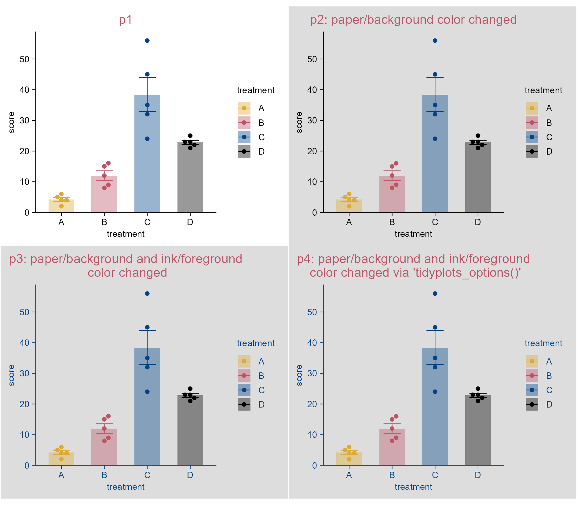
library(tidyplots)
# View top 10 rows of the columns used
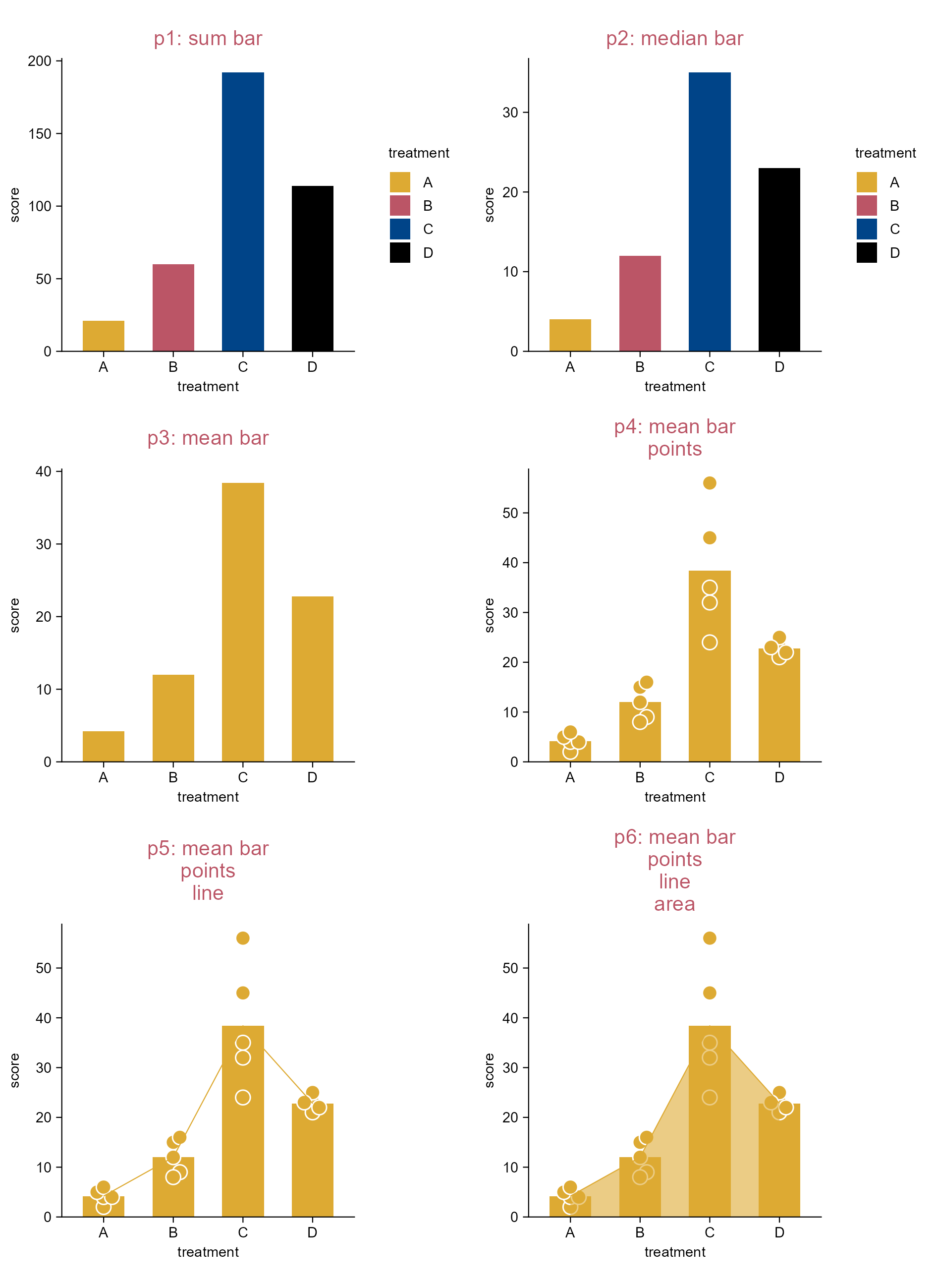
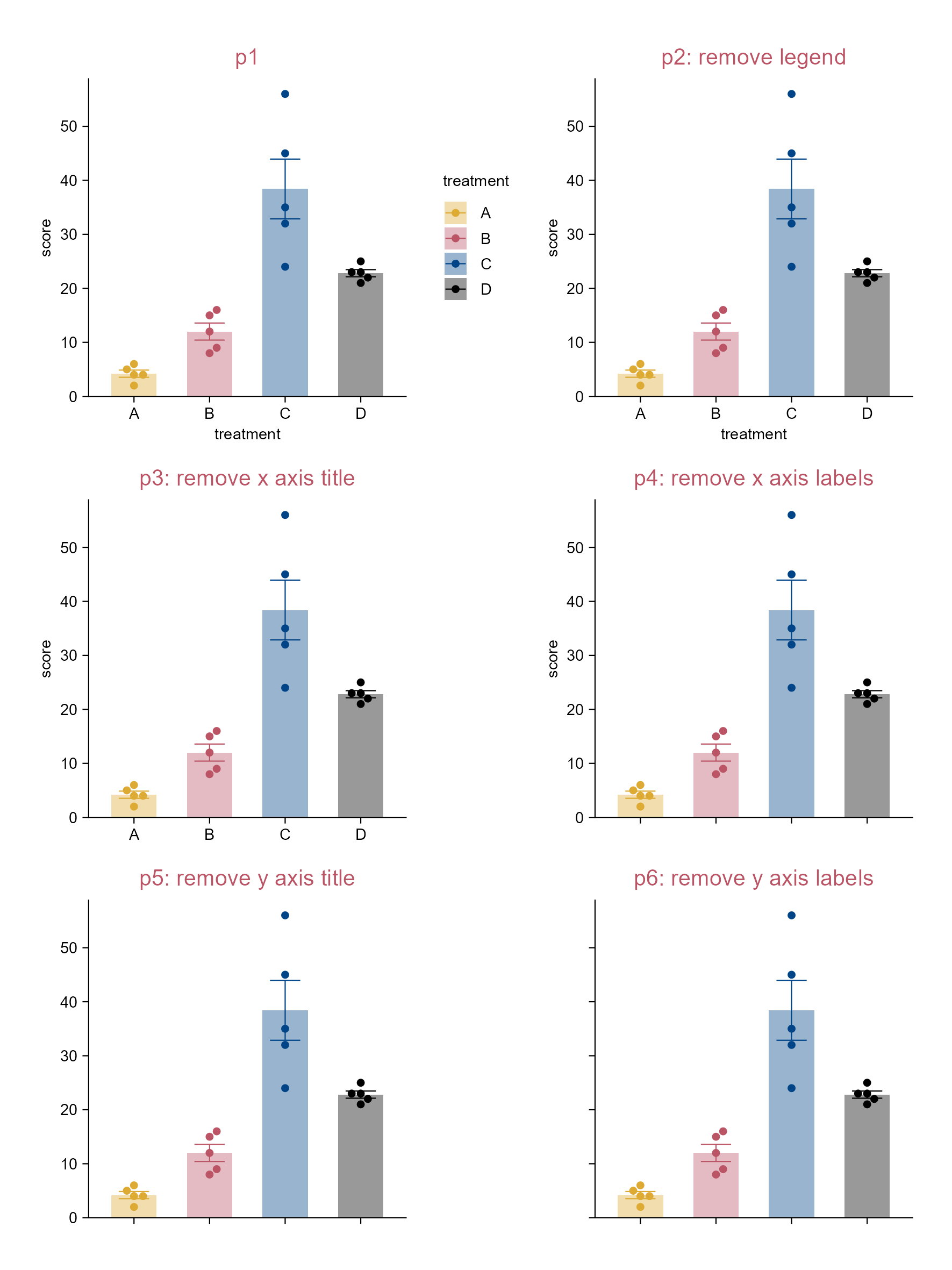
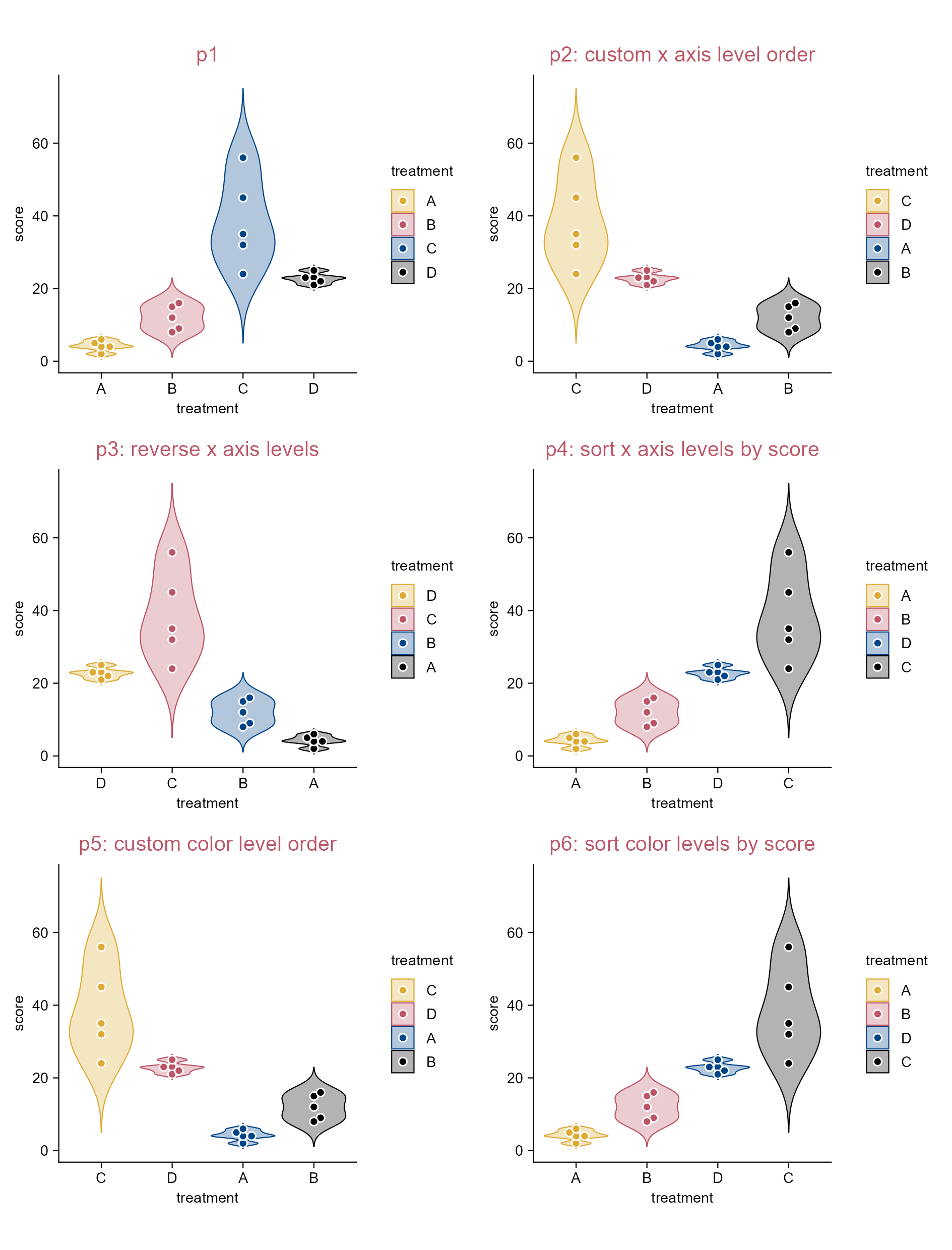
study |>
dplyr::select(treatment, score) |>
dplyr::slice_head(n = 10)# A tibble: 10 × 2
treatment score
<chr> <dbl>
1 A 2
2 A 4
3 A 5
4 A 4
5 A 6
6 B 9
7 B 8
8 B 12
9 B 15
10 B 16