# The intended width of image in plot
img_intend_width = 50 # unit: mm
# Tailor relative extra spaces of plot (0 (0%) - 1 (100%))
top_extra = 0.12; right_extra = 0; bottom_extra = 0; left_extra = 0.16
# The width and height of plot
plot_width = img_intend_width * (1 + left_extra + right_extra) # unit: mm
plot_height = img_intend_width * (img_height/img_width) * (1 + top_extra + bottom_extra)
# Plot
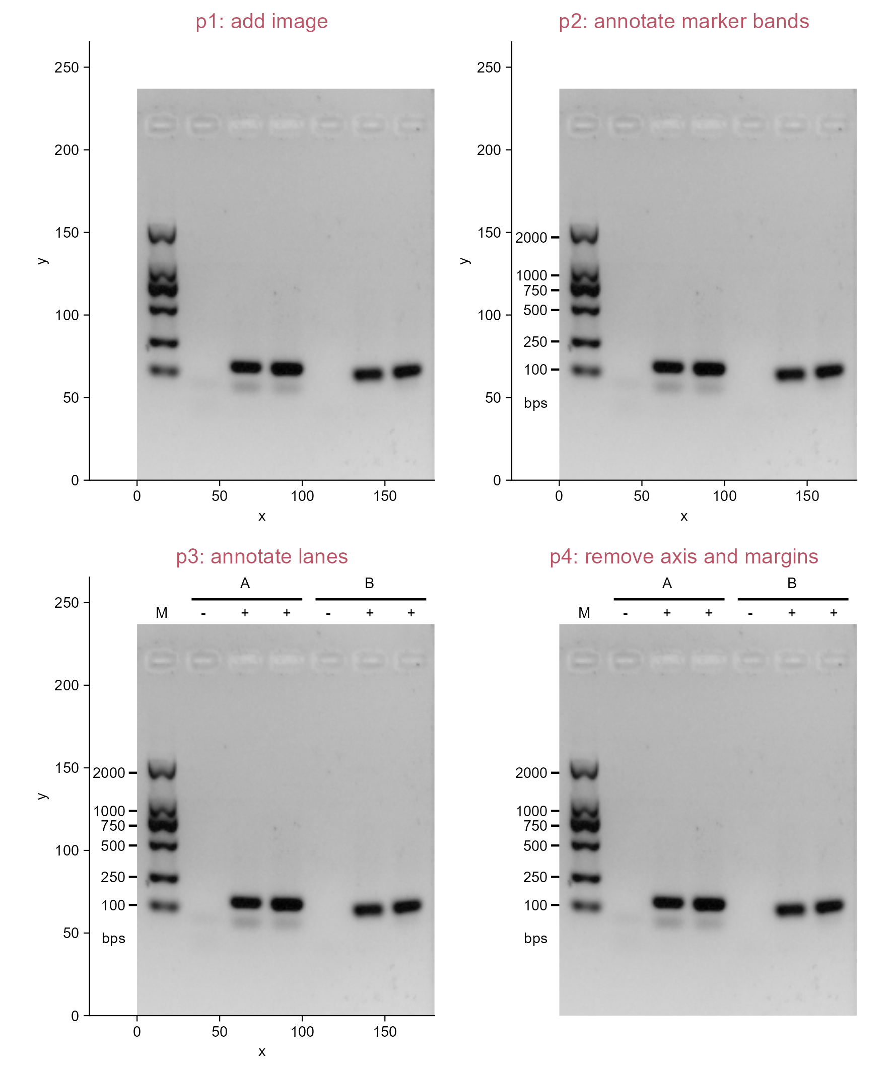
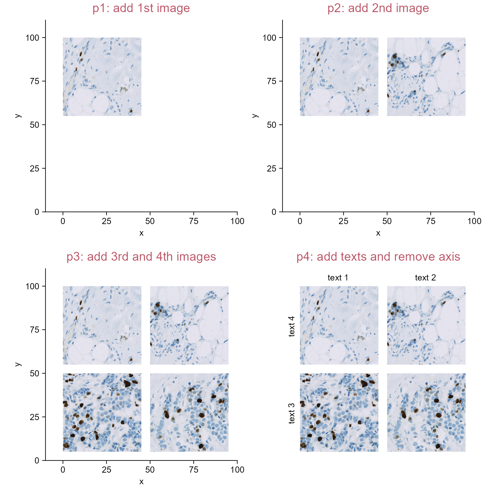
p1 <- df |> tidyplot(x = x, y = y) |>
add_data_points(alpha = 0) |>
add(ggplot2::annotation_custom(img_grob, xmin = 0, xmax = img_width,
ymin = 0, ymax = img_height)) |>
add_title(title = "p1: add image") |>
adjust_size(width = plot_width, height = plot_height) |>
adjust_x_axis(limits = c(-img_width*left_extra, img_width*(1 + right_extra))) |>
adjust_y_axis(limits = c(-img_height * bottom_extra, img_height * (1 + top_extra)))
p2 <- p1 |>
adjust_title(title = "p2: annotate marker bands") |>
add_annotation_line(x = 0, xend = -5,
y = img_height - c(90, 113, 122, 134, 153, 170), # numbers are obtained via ImageJ
yend = img_height - c(90, 113, 122, 134, 153, 170)) |>
add_annotation_text(text = c("2000", "1000", "750", "500", "250", "100", "bps"),
x = -7, y = img_height - c(90, 113, 122, 134, 153, 170, 190), hjust = 1)
p3 <- p2 |>
adjust_title(title = "p3: annotate lanes") |>
add_annotation_line(x = c(33, 108), xend = c(100, 175),
y = img_height + 15, yend = img_height + 15) |>
add_annotation_text(text = c("A", "B"), x = c(65.3, 140.8), y = img_height + 25) |>
add_annotation_text(text = c("M", "-", "+", "+", "-", "+", "+"),
x = seq(15, 166, length.out = 7), y = img_height + 7)
p4 <- p3 |>
adjust_title(title = "p4: remove axis and margins") |>
remove_x_axis() |> remove_y_axis() |>
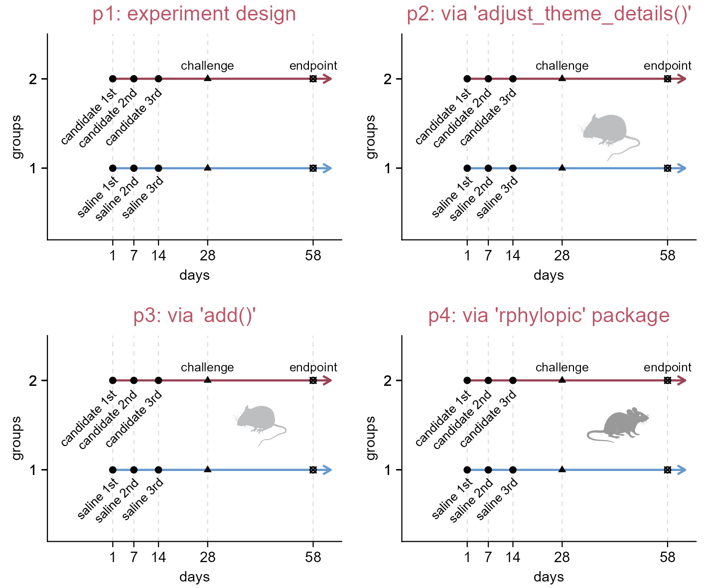
adjust_theme_details(plot.margin = ggplot2::margin(0, 0, 0, 0))