5  Additional plot types and techniques

5.1 Violin plot

library(tidyplots)

# View top 10 rows of the columns used
study |> 
  dplyr::select(treatment, score) |> 
  dplyr::slice_head(n = 10)
# A tibble: 10 × 2
   treatment score
   <chr>     <dbl>
 1 A             2
 2 A             4
 3 A             5
 4 A             4
 5 A             6
 6 B             9
 7 B             8
 8 B            12
 9 B            15
10 B            16
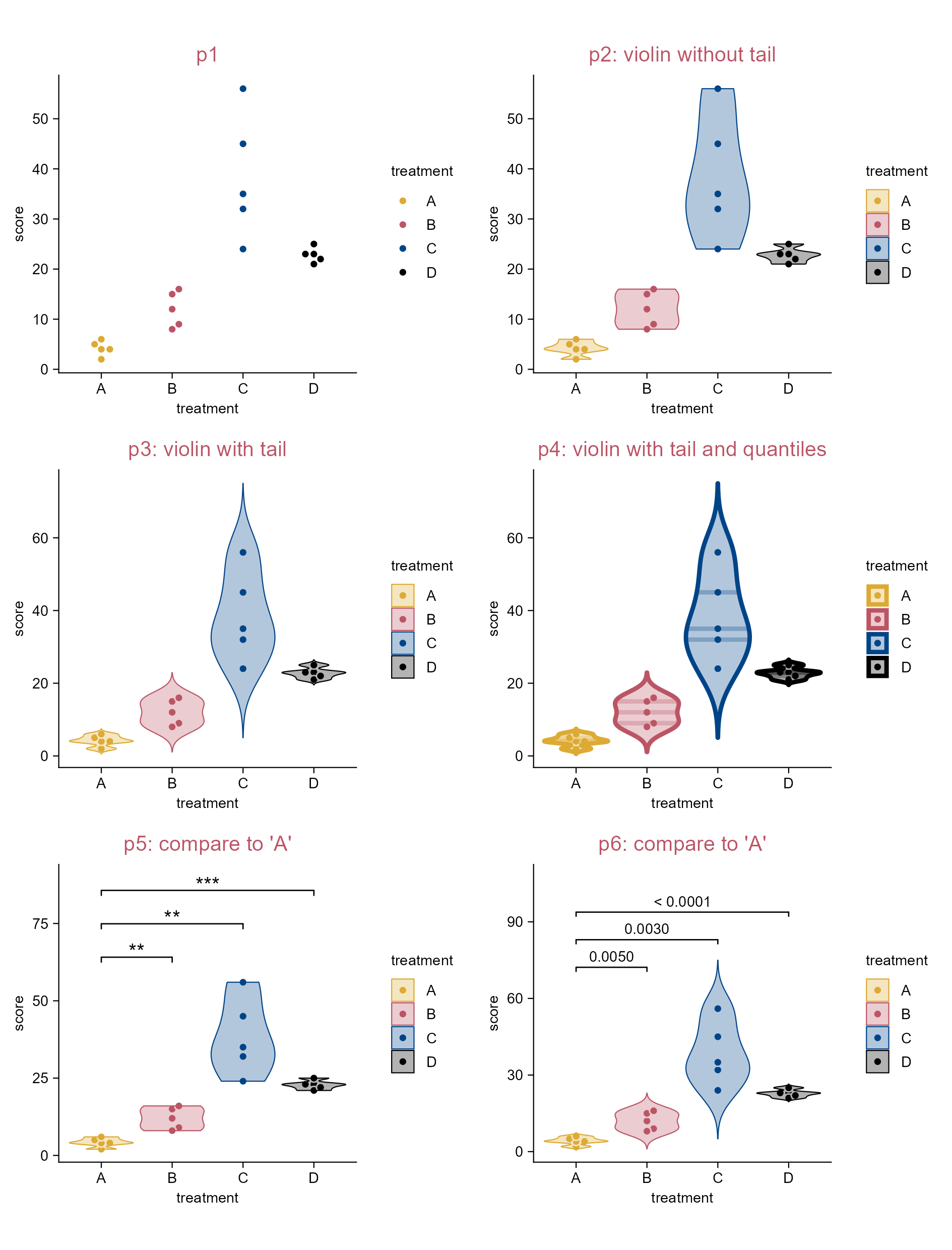
# Plot
p1 <- study |> 
  tidyplot(x = treatment, y = score, color = treatment) |> 
  add_data_points_beeswarm(white_border = TRUE) |> 
  add_title(title = "p1")

p2 <- p1 |> 
  adjust_title(title = "p2: violin without tail") |> 
  add_violin()

p3 <- p1 |> 
  adjust_title(title = "p3: violin with tail") |> 
  add_violin(trim = FALSE)

p4 <- p1 |> 
  adjust_title(title = "p4: violin with tail and quantiles") |> 
  add_violin(
    trim = FALSE, 
    quantile.linetype = "solid", 
    linewidth = 1)

p5 <- p2 |> 
  adjust_title(title = "p5: compare to 'A'") |> 
  add_test_asterisks(ref.group = "A", hide_info = TRUE)

p6 <- p3 |> 
  adjust_title(title = "p6: compare to 'A'") |> 
  add_test_pvalue(ref.group = "A", padding_top = 0.2, 
    bracket.nudge.y = 0.3, step.increase = 0.2, hide_info = TRUE)

Violin plot.

5.2 (Rasterize) correlation heatmap

library(tidyplots)

df <- "https://tidyplots.org/data/correlation-matrix.csv" |> 
  readr::read_csv(show_col_types = FALSE)
df |> dim()
[1] 202500      5
# View top 10 rows of the columns used
df |> dplyr::select(x, y, correlation) |> 
  dplyr::slice_head(n = 10)
# A tibble: 10 × 3
   x       y       correlation
   <chr>   <chr>         <dbl>
 1 YAL022C YAL022C      1     
 2 YAL022C YAL040C      0.505 
 3 YAL022C YAL053W      0.0730
 4 YAL022C YAL067C     -0.244 
 5 YAL022C YAR003W      0.0282
 6 YAL022C YAR007C     -0.197 
 7 YAL022C YAR008W     -0.0395
 8 YAL022C YAR018C      0.692 
 9 YAL022C YBL002W     -0.0289
10 YAL022C YBL003C     -0.125 
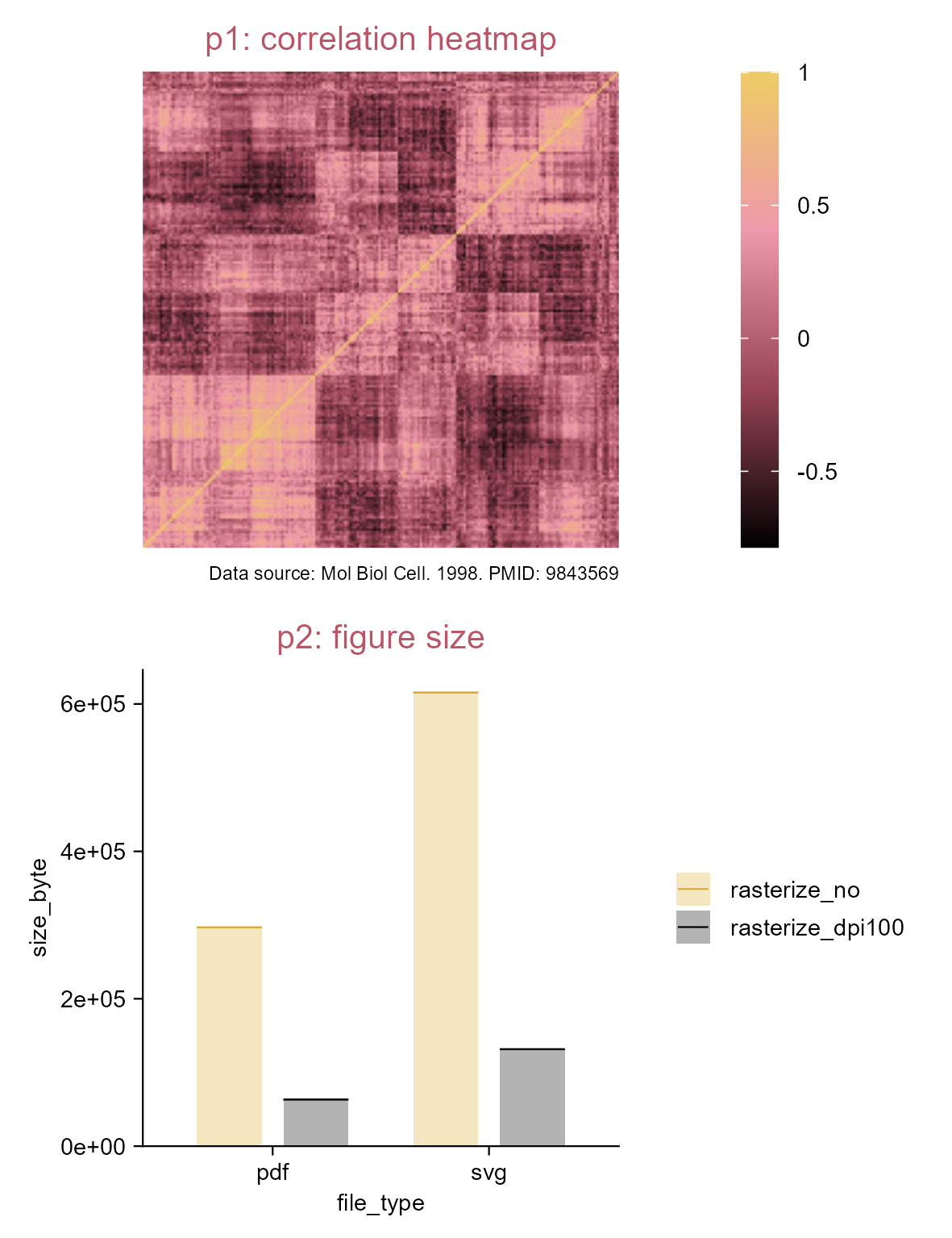
# Plot
p0 <- df |> 
  tidyplot(x = x, y = y, color = correlation) |>    
  remove_legend_title() |> 
  adjust_theme_details(legend.key.height = ggplot2::unit(1, "null"),
    legend.margin = ggplot2::margin_part(t = 0, b = 0)) |> 
  add(ggplot2::scale_fill_gradient2(
    low = "#994455", mid = "#ffffff", high = "#004488", 
    midpoint = 0)) |> 
  add_caption("Data source: Mol Biol Cell. 1998. PMID: 9843569")

# Save vector images without rasterization
p0 |> 
  add_heatmap() |> 
  sort_x_axis_levels(order_x) |> sort_y_axis_levels(order_y) |> 
  remove_x_axis() |> remove_y_axis() |> 
  save_plot("images/rasterize_correlation_no.pdf", view_plot = FALSE) |> 
  save_plot("images/rasterize_correlation_no.svg", view_plot = FALSE)

# Save vector images with rasterization (dpi = 100)
p0 |> 
  add_heatmap(rasterize = TRUE, rasterize_dpi = 100) |> 
  sort_x_axis_levels(order_x) |> sort_y_axis_levels(order_y) |> 
  remove_x_axis() |> remove_y_axis() |> 
  save_plot("images/rasterize_correlation_yes_dpi100.pdf", view_plot = FALSE) |> 
  save_plot("images/rasterize_correlation_yes_dpi100.svg", view_plot = FALSE)

List the figures saved:

images
├── rasterize_correlation_no.pdf
├── rasterize_correlation_no.svg
├── rasterize_correlation_yes_dpi100.pdf
└── rasterize_correlation_yes_dpi100.svg

Rasterize correlation heatmap selectively.

5.3 Heatmap (z-score)

Tip

This is expecially useful when you want to focus on the dynamics within rows or columns.

library(tidyplots)

# View top 10 rows of the columns used
climate |> 
  dplyr::select(month, year, max_temperature) |> 
  dplyr::slice_head(n = 10)
# A tibble: 10 × 3
   month  year max_temperature
   <chr> <dbl>           <dbl>
 1 01     1891           -1.49
 2 02     1891            3.37
 3 03     1891            5.05
 4 04     1891            8.34
 5 05     1891           16.2 
 6 06     1891           18.2 
 7 07     1891           20.5 
 8 08     1891           18.2 
 9 09     1891           18.3 
10 10     1891           14.2 
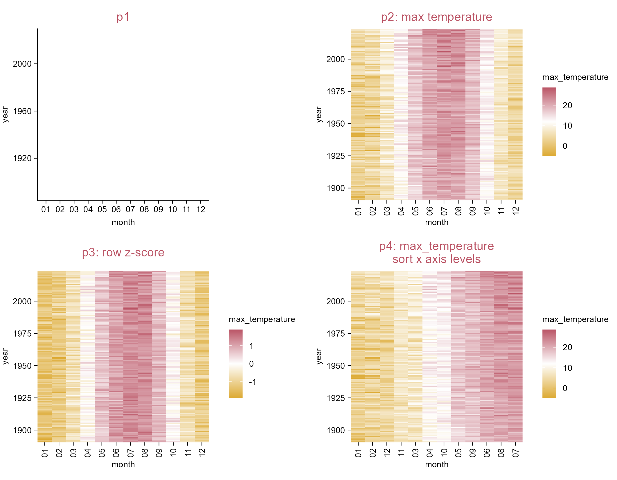
# Plot
p1 <- climate |> 
  tidyplot(
    x = month, 
    y = year, 
    color = max_temperature) |> 
  add_title("p1")

p2 <- p1 |> 
  add_heatmap() |>  
  adjust_colors(
    new_colors = c(
      "#f7f8f9", 
      "#004488")) |>
  adjust_title("p2: max temperature")

p3 <- p1 |> 
  add_heatmap(scale = "row") |> 
  adjust_colors(new_colors = c(
    "#994455", 
    "#ffffff", 
    "#004488")) |> 
  adjust_title("p3: row z-score")

p4 <- p2 |> 
  sort_x_axis_levels(max_temperature) |>
  adjust_title(
    paste(
      "p4: max_temperature", 
      "sort x axis levels", 
      sep = "\n"))

Heatmap_z-scores.

5.4 (Rasterize) volcano plot

library(tidyplots)

df <- 
  "https://tidyplots.org/data/differential-expression-analysis.csv" |> 
  readr::read_csv(show_col_types = FALSE) |> 
  dplyr::mutate(
    neg_log10_padj = -log10(padj),
    direction = dplyr::if_else(log2FoldChange > 0, "up", "down", "NA"),
    candidate = abs(log2FoldChange) >= 1 & padj < 0.05)
df |> dim()
[1] 43629    17
# View top 10 rows of the columns used
df |> 
  dplyr::select(
    log2FoldChange, neg_log10_padj, candidate, 
    direction, padj, external_gene_name) |> 
  dplyr::slice_head(n = 10)
# A tibble: 10 × 6
   log2FoldChange neg_log10_padj candidate direction     padj external_gene_name
            <dbl>          <dbl> <lgl>     <chr>        <dbl> <chr>             
 1         -0.989         0.642  FALSE     down       2.28e-1 Gnai3             
 2         NA            NA      NA        <NA>      NA       Pbsn              
 3          0.342         0.0913 FALSE     up         8.10e-1 Cdc45             
 4          0.865         0.322  FALSE     up         4.77e-1 H19               
 5         -0.998         0.284  FALSE     down       5.20e-1 Scml2             
 6         -1.47          0.458  FALSE     down       3.48e-1 Apoh              
 7         -0.696         0.539  FALSE     down       2.89e-1 Narf              
 8         -2.52          4.02   TRUE      down       9.52e-5 Cav2              
 9         -1.26          2.04   TRUE      down       9.06e-3 Klf6              
10         -0.648         0.317  FALSE     down       4.82e-1 Scmh1             
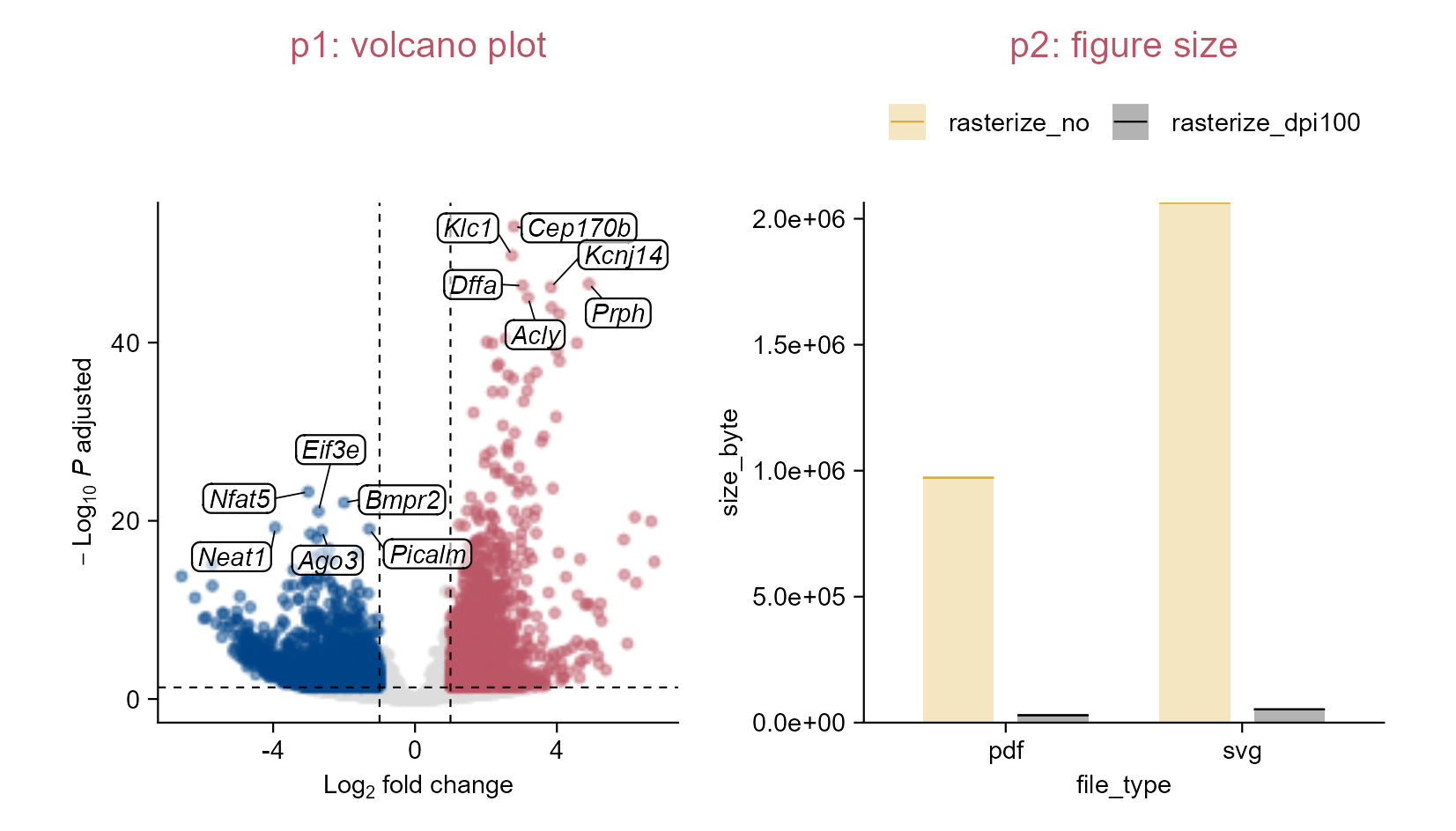
p0 <- df |> 
  tidyplot(x = log2FoldChange, y = neg_log10_padj) |> 
  add_data_labels_repel(
    data = min_rows(padj, 6, by = direction), 
    label = external_gene_name, 
    color = "#000000", 
    min.segment.length = 0, 
    background = TRUE, 
    fontface = "italic") |> 
  adjust_x_axis_title("$Log[2]~fold~change$") |> 
  adjust_y_axis("$-Log[10]~italic(P)~adjusted$")

# Save vector images without rasterization
p0 |> 
  add_data_points(data = filter_rows(!candidate), color = "#dddddd") |> 
  add_data_points(
    data = filter_rows(candidate, direction == "up"), 
    color = "#bb5566", alpha = 0.5) |> 
  add_data_points(
    data = filter_rows(candidate, direction == "down"), 
    color = "#004488", alpha = 0.5) |>   
  add_reference_lines(x = c(-1, 1), y = -log10(0.05)) |> 
  save_plot("images/rasterize_volcano_no.pdf", view_plot = FALSE) |> 
  save_plot("images/rasterize_volcano_no.svg", view_plot = FALSE)

# Save vector images with rasterization (dpi = 100)
p0 |>   
  add_data_points(data = filter_rows(!candidate), color = "#dddddd", 
  rasterize = TRUE, rasterize_dpi = 100) |> 
  add_data_points(
    data = filter_rows(candidate, direction == "up"), color = "#bb5566", 
    alpha = 0.5, rasterize = TRUE, rasterize_dpi = 100) |> 
  add_data_points(
    data = filter_rows(candidate, direction == "down"), color = "#004488", 
    alpha = 0.5, rasterize = TRUE, rasterize_dpi = 100) |>   
  add_reference_lines(x = c(-1, 1), y = -log10(0.05)) |> 
  save_plot("images/rasterize_volcano_yes_dpi100.pdf", view_plot = FALSE) |> 
  save_plot("images/rasterize_volcano_yes_dpi100.svg", view_plot = FALSE)

List the figures saved:

images
├── rasterize_correlation_no.pdf
├── rasterize_correlation_no.svg
├── rasterize_correlation_yes_dpi100.pdf
└── rasterize_correlation_yes_dpi100.svg

Rasterize volcano plot selectively.

5.5 Lollipop plot

library(tidyplots)

# View top 10 rows of the columns used
spendings |> 
  dplyr::select(amount, category) |> 
  dplyr::slice_head(n = 10)
# A tibble: 10 × 2
   amount category      
    <dbl> <chr>         
 1    100 Food          
 2     40 Transportation
 3   1200 Housing       
 4     80 Utilities     
 5     75 Education     
 6    200 Insurance     
 7     60 Food          
 8     50 Utilities     
 9     90 Food          
10     40 Transportation
# Plot
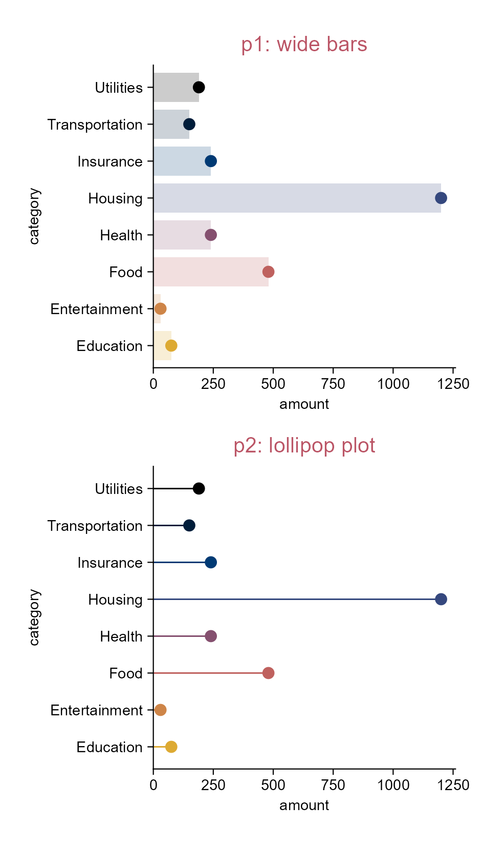
p1 <- spendings |> 
  tidyplot(
    x = amount, 
    y = category, 
    color = category) |> 
  add_sum_bar(
    width = 0.8, 
    alpha = 0.2) |> 
  add_sum_dot() |> 
  add_title("p1: wide bars") |> 
  remove_legend()

p2 <- spendings |> 
  tidyplot(
    x = amount, 
    y = category, 
    color = category) |> 
  add_sum_bar(
    width = 0.05, 
    alpha = 1) |> 
  add_sum_dot() |> 
  add_title("p2: lollipop plot") |> 
  remove_legend()

Lollipop plot.
Tip

In essence, lollipop plot is generated via narrowing down bar width.

5.6 Dumbbell plot

library(tidyplots)

# View top 10 rows of the columns used
study |> 
  dplyr::select(participant, score, group) |> 
  dplyr::slice_head(n = 10)
# A tibble: 10 × 3
   participant score group  
   <chr>       <dbl> <chr>  
 1 p01             2 placebo
 2 p02             4 placebo
 3 p03             5 placebo
 4 p04             4 placebo
 5 p05             6 placebo
 6 p06             9 placebo
 7 p07             8 placebo
 8 p08            12 placebo
 9 p09            15 placebo
10 p10            16 placebo
# Plot
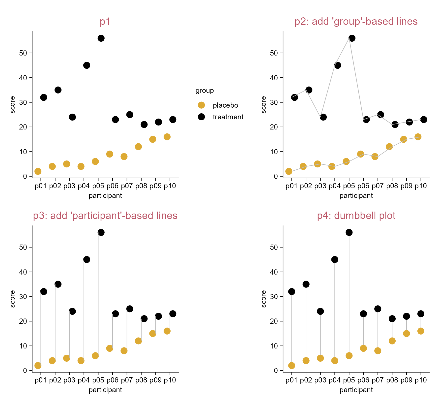
p1 <- study |> 
  tidyplot(
    x = participant, 
    y = score, 
    color = group) |> 
  add_data_points(size = 2.5) |> 
  add_title(title = "p1")

p2 <- p1 |> 
  adjust_title(title = "p2: add 'group'-based lines") |>  
  add_line(color = "#bbbbbb")

p3 <- p1 |> 
  adjust_title(title = "p3: add 'participant'-based lines") |> 
  add_line(
    group = participant, 
    color = "#bbbbbb")

p4 <- study |> 
  tidyplot(
    x = participant, 
    y = score, 
    color = group, 
    dodge_width = 0) |> 
  add_title(title = "p4: dumbbell plot") |> 
  add_line(
    group = participant, 
    color = "#bbbbbb") |> 
  add_data_points(size = 2.5)

Dumbbell plot.

5.7 Dumbbell plot with data labels

library(tidyplots)

# Calculation
study_fct <- study |> # ensure the same order for `participant` and its levels
  dplyr::arrange(group, rev(participant)) |> 
  dplyr::mutate(participant = forcats::fct_inorder(participant))

# View top 5 rows of the columns used
study_fct |> 
  dplyr::select(participant, score, group) |> 
  dplyr::slice_head(n = 5)
# A tibble: 5 × 3
  participant score group  
  <fct>       <dbl> <chr>  
1 p10            16 placebo
2 p09            15 placebo
3 p08            12 placebo
4 p07             8 placebo
5 p06             9 placebo
# Plot
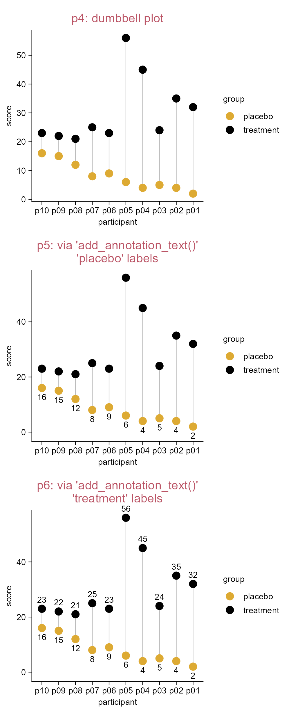
p4 <- study_fct |> # from last section but with reversed x levels
  tidyplot(
    x = participant, 
    y = score, 
    color = group, 
    dodge_width = 0) |> 
  add_title(title = "p4: dumbbell plot") |> 
  add_line(
    group = participant, 
    color = "#bbbbbb") |> 
  add_data_points(size = 2.5)

p5 <- p4 |> 
  add_title(title = "p5: via 'add_annotation_text()'\n'placebo' labels") |> 
  add_annotation_text(
    text = study_fct$score[study_fct$group == "placebo"], 
    x = 1:10, # see the note of next page
    y = study_fct$score[study_fct$group == "placebo"], 
    vjust = 2) |> # tailored value
  remove_clipping() |> 
  adjust_padding(bottom = 0.1) # to accommodate the labels for the "placebo" group

p6 <- p5 |> 
  add_title(title = "p6: via 'add_annotation_text()'\n'treatment' labels") |> 
  add_annotation_text(
    text = study_fct$score[study_fct$group == "treatment"], 
    x = 1:10, # see note
    y = study_fct$score[study_fct$group == "treatment"],
    vjust = -1) # tailored value

Dumbbell plot with data labels.
Note

Internally, ggplot2 (and of course tidyplots) handles discrete scales by mapping each category to an integer value and then drawing the geom at the corresponding coordinate location. https://ggplot2-book.org/scales-position.html#sec-discrete-position

5.8 Pie and donut plots

library(tidyplots)

# View top 10 rows of the columns used
energy |> 
  dplyr::select(energy, energy_source) |> 
  dplyr::slice_head(n = 10)
# A tibble: 10 × 2
    energy energy_source              
     <dbl> <fct>                      
 1   3.72  Biomass                    
 2 141.    Fossil brown coal / lignite
 3  40.0   Fossil gas                 
 4 111.    Fossil hard coal           
 5   1.76  Fossil oil                 
 6   0     Geothermal                 
 7  23.4   Hydro                      
 8 156.    Nuclear                    
 9   6.31  Others                     
10   0.196 Solar                      
# Plot
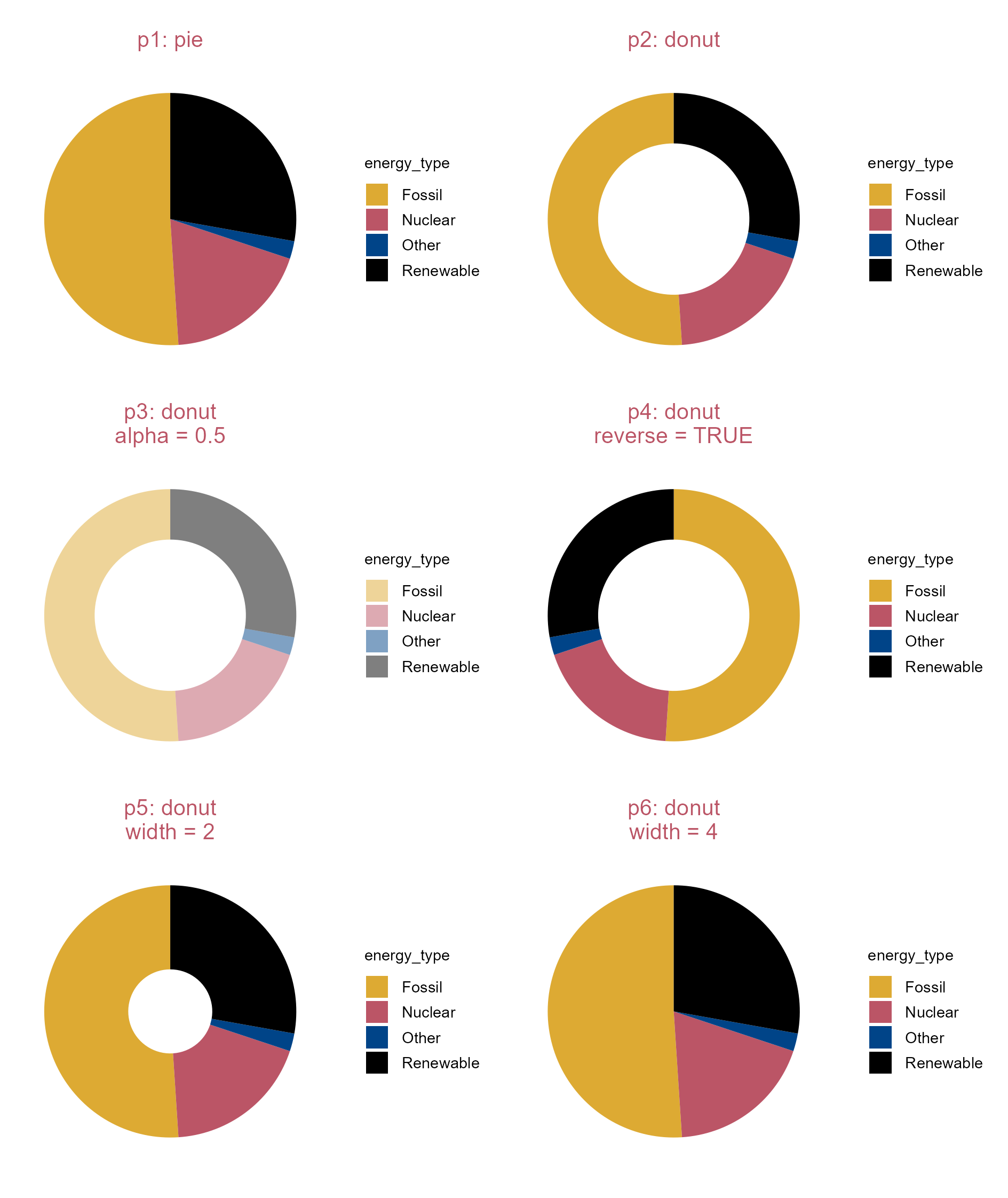
p0 <- energy |> 
  tidyplot(
    y = energy, 
    color = energy_type)

p1 <- p0 |> 
  add_pie() |> 
  add_title(title = "p1: pie")

p2 <- p0 |>  
  add_donut() |> 
  add_title(title = "p2: donut")

p3 <- p0 |> 
  add_donut(alpha = 0.5) |> 
  add_title(title = paste("p3: donut", "alpha = 0.5", sep = "\n"))

p4 <- p0 |> 
  add_donut(reverse = TRUE) |> 
  add_title(title = paste("p4: donut", "reverse = TRUE", sep = "\n"))

p5 <- p0 |> 
  add_donut(width = 2) |> 
  add_title(title = paste("p5: donut", "width = 2", sep = "\n"))

p6 <- p0 |> 
  add_donut(width = 4) |> 
  add_title(title = paste("p6: donut", "width = 4", sep = "\n"))

Pie and donut plots.

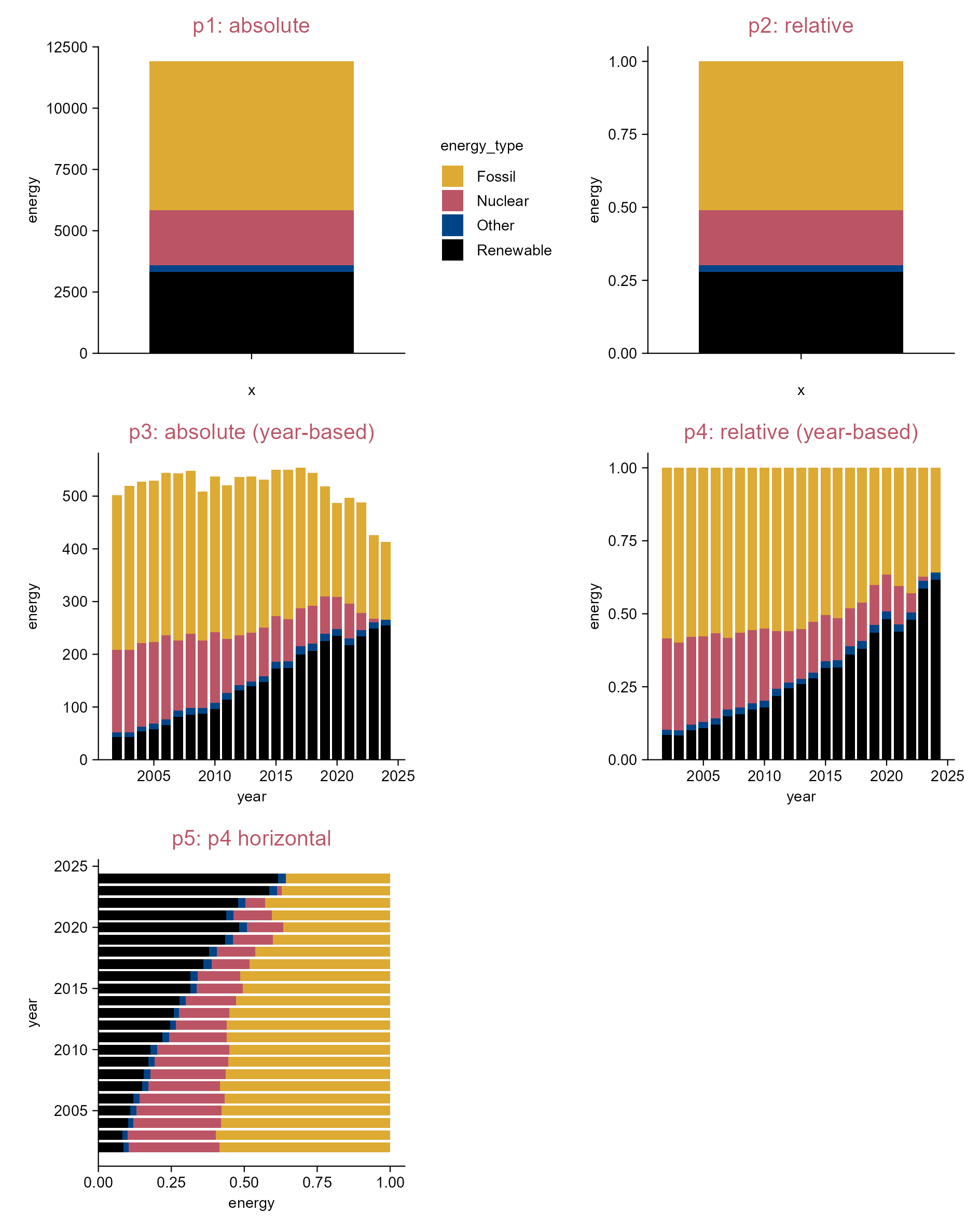
5.9 Stacked bar plot

library(tidyplots)

# View top 10 rows of the columns used
energy |> 
  dplyr::select(year, energy, energy_type) |> 
  dplyr::slice_head(n = 10)
# A tibble: 10 × 3
    year  energy energy_type
   <dbl>   <dbl> <fct>      
 1  2002   3.72  Renewable  
 2  2002 141.    Fossil     
 3  2002  40.0   Fossil     
 4  2002 111.    Fossil     
 5  2002   1.76  Fossil     
 6  2002   0     Renewable  
 7  2002  23.4   Renewable  
 8  2002 156.    Nuclear    
 9  2002   6.31  Other      
10  2002   0.196 Renewable  
# Plot
p1 <- energy |> 
  tidyplot(y = energy, color = energy_type) |> 
  add_title(title = "p1: absolute") |> 
  add_barstack_absolute()

p2 <- energy |> 
  tidyplot(y = energy, color = energy_type) |> 
  add_title(title = "p2: relative") |> 
  add_barstack_relative() |> 
  remove_legend()

p3 <- energy |> 
  tidyplot(x = year, y = energy, color = energy_type) |> 
  add_title(title = "p3: absolute (year-based)") |> 
  add_barstack_absolute() |>
  remove_legend()  

p4 <- energy |> 
  tidyplot(x = year, y = energy, color = energy_type) |> 
  add_title(title = "p4: relative (year-based)") |> 
  add_barstack_relative() |>
  remove_legend() 

p5 <- energy |> 
  tidyplot(x = energy, y = year, color = energy_type) |> 
  add_title(title = "p5: p4 horizontal") |> 
  add_barstack_relative(orientation = "y") |> 
  remove_legend()

Stacked bar plot.

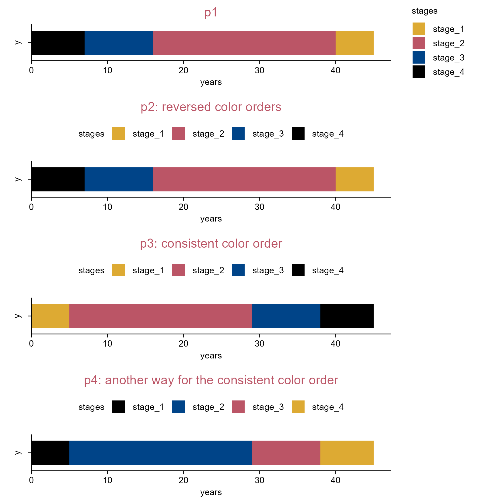
5.10 Consistent color order between the horizontal stacked bar and the legend

library(tidyplots)

# A putative df
stages <- c("stage_1", "stage_2", "stage_3", "stage_4")
years = c(5, 24, 9, 7)

df <- tibble::tibble(
  years = years,
  stages = stages)

# View
df
# A tibble: 4 × 2
  years stages 
  <dbl> <chr>  
1     5 stage_1
2    24 stage_2
3     9 stage_3
4     7 stage_4
# Plot
p0 <- df |> 
  tidyplot(
    x = years, 
    color = stages, 
    width = 100, 
    height = 10)

p1 <- p0 |> 
  add_barstack_absolute() |> 
  add_title(title = "p1")

p2 <- p0 |>
  add_barstack_absolute() |> 
  adjust_title(title = "p2: reversed color orders") |> 
  adjust_legend_position(position = "top")

p3 <- p0 |>   
  add_barstack_absolute(reverse = TRUE) |> 
  add_title(title = "p3: consistent color order") |> 
  adjust_legend_position(position = "top")

p4 <- p0 |> 
  add_barstack_absolute() |> 
  add_title(title = "p4: another way for the consistent color order") |> 
  adjust_legend_position(position = "top") |> 
  add(ggplot2::guides(fill = ggplot2::guide_legend(reverse = TRUE))) |> 
  reverse_color_levels()

Consistent color order between the horizontal stacked bar and the legend.
Note

The color mappings in p3 and p4 are reversed.

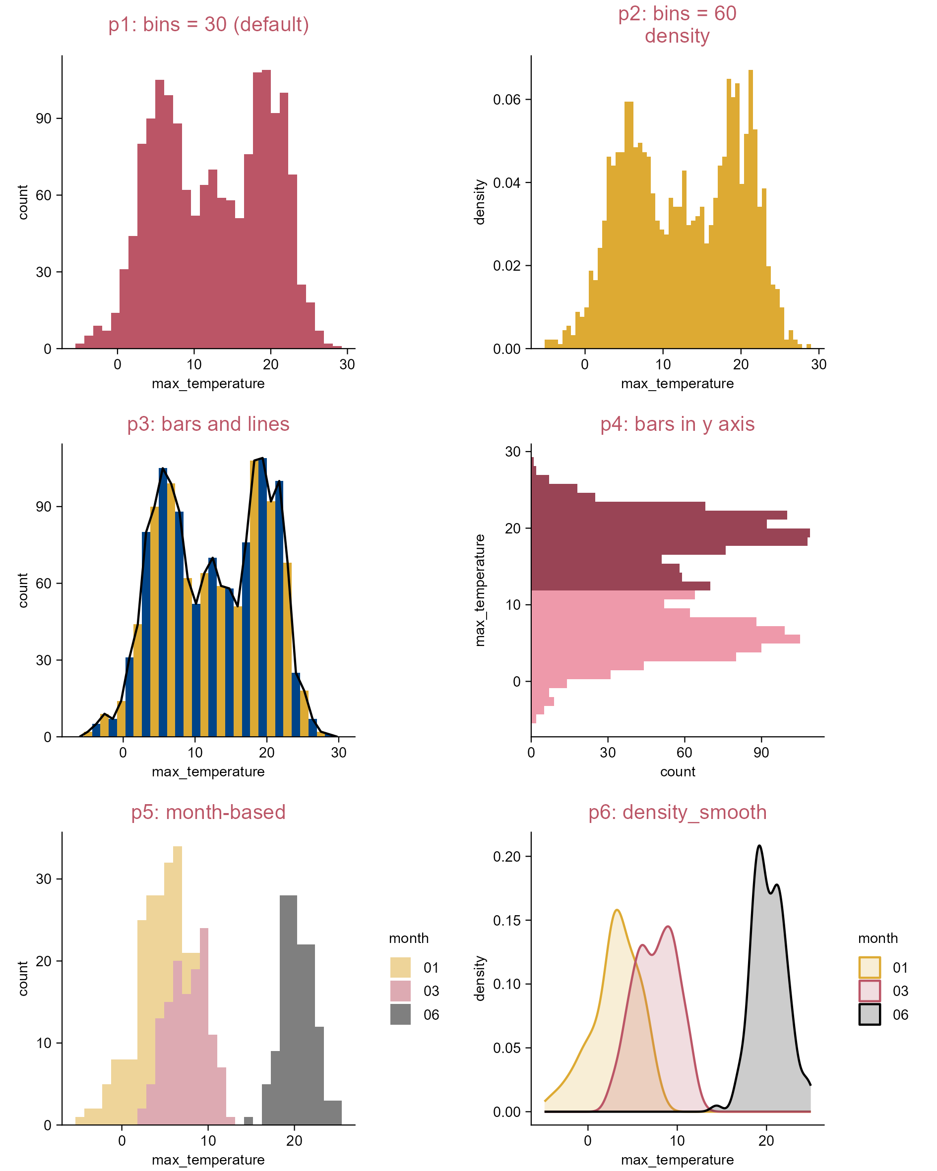
5.11 Histogram

library(tidyplots)

# View top 10 rows of the columns used
climate |> 
  dplyr::select(max_temperature, month) |> 
  dplyr::slice_head(n = 10)
# A tibble: 10 × 2
   max_temperature month
             <dbl> <chr>
 1           -1.49 01   
 2            3.37 02   
 3            5.05 03   
 4            8.34 04   
 5           16.2  05   
 6           18.2  06   
 7           20.5  07   
 8           18.2  08   
 9           18.3  09   
10           14.2  10   
# Plot
p0 <- climate |> 
  tidyplot(x = max_temperature)

p1 <- p0 |> 
  add_title(title = "p1: bins = 30 (default)") |> 
  add_histogram(color = "#bb5566")

p2 <- p0 |> 
  add_title(title = paste("p2: bins = 60", "density", sep = "\n")) |> 
  add_histogram(bins = 60, mapping = ggplot2::aes(y = ggplot2::after_stat(density)))

p3 <- p0 |>
  add_histogram(color = rep(c("#ddaa33", "#004488"), length.out = 30)) |> 
  adjust_title(title = "p3: bars and lines") |> 
  add(ggplot2::geom_freqpoly(bins = 30, color = "#000000"))

p4 <- climate |> 
  tidyplot(y = max_temperature) |>   
  add_title(title = "p4: bars in y axis") |> 
  add_histogram(color = rep(c("#ee99aa", "#994455"), each  = 15))

p5 <- climate |> 
  dplyr::filter(month %in% c("01", "03", "06")) |> 
  tidyplot(x = max_temperature, color = month) |> 
  add_title(title = "p5: month-based") |> 
  add_histogram(
    alpha = 0.5, 
    position = "identity") # "stack" in default

p6 <- climate |> 
  dplyr::filter(month %in% c("01", "03", "06")) |> 
  tidyplot(x = max_temperature, color = month) |> 
  add_title(title = "p6: density_smooth") |> 
  add(ggplot2::geom_density(alpha = 0.2))

Histogram.

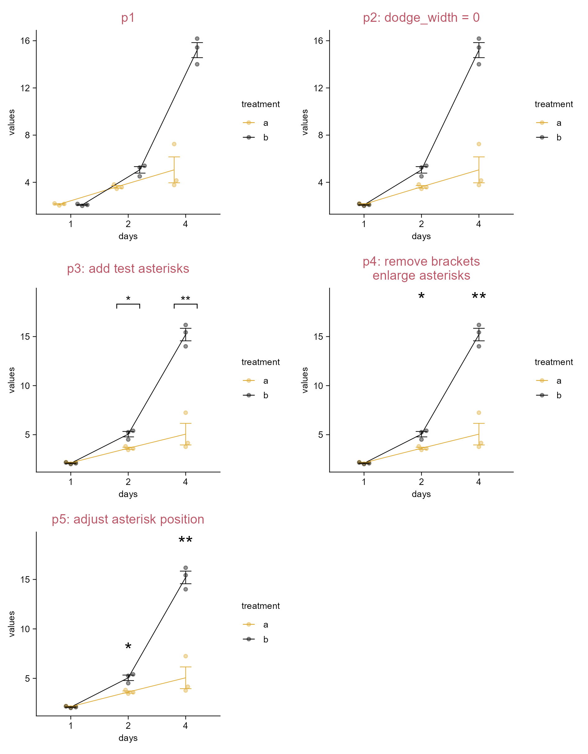
5.12 Line plot

library(tidyplots)

set.seed(2026) # for repeatability

# Create a putative df
df <- tibble::tibble(
  values = c(
    runif(n = 6, min = 2, max = 2.3),
    runif(n = 3, min = 3.3, max = 3.9),
    runif(n = 3, min = 4.5, max = 5.8),
    runif(n = 3, min = 3, max = 8),
    runif(n = 3, min = 14, max = 18)),
  treatment = rep(c("a", "b"), each = 3, times = 3),
  days = factor(rep(c(1, 2, 4), each = 6))) # factor

# View top 10 rows of the columns used
df |> dplyr::slice_head(n = 10)
# A tibble: 10 × 3
   values treatment days 
    <dbl> <chr>     <fct>
 1   2.21 a         1    
 2   2.17 a         1    
 3   2.04 a         1    
 4   2.09 b         1    
 5   2.17 b         1    
 6   2.01 b         1    
 7   3.58 a         2    
 8   3.82 a         2    
 9   3.45 a         2    
10   5.26 b         2    
# Plot
p1 <- df |> 
  tidyplot(x = days, y = values, color = treatment) |> 
  add_data_points_beeswarm(alpha = 0.4) |> 
  add_mean_line() |> add_sem_errorbar() |> add_title(title = "p1")

p2 <- df |> 
  tidyplot(x = days, y = values, color = treatment, dodge_width = 0) |> 
  add_data_points_beeswarm(alpha = 0.4) |> 
  add_mean_line() |> add_sem_errorbar() |> add_title(title = "p2: dodge_width = 0")

p3 <- p2 |> 
  adjust_title(title = "p3: add test asterisks") |> 
  add_test_asterisks(hide_info = TRUE)

p4 <- p2 |> 
  adjust_title(title = "p4: remove brackets\nenlarge asterisks") |> 
  add_test_asterisks(
    hide_info = TRUE,
    label.size = 15/ggplot2::.pt,
    remove.bracket = TRUE)

df_day2 <- df |> dplyr::filter(days == 2)
df_day4 <- df |> dplyr::filter(days == 4)

p5 <- p2 |> 
  add_title(title = "p5: adjust asterisk position") |> 
  add_test_asterisks(
    hide_info = TRUE,
    label.size = 15/ggplot2::.pt,
    remove.bracket = TRUE,
    y.position = c(
      max(df_day2$values) + 2, # 2 is a tailored number
      max(df_day4$values) + 2))

Line plot.