2  Plots

2.1 Overview of plots

library(tidyplots)

p1 <- study |> 
  tidyplot(x = treatment, y = score, color = treatment) |> 
  add_title(title = "p1") |> 
  add_violin(trim = FALSE) |> 
  add_sem_errorbar() |> 
  add_data_points_beeswarm()

p2 <- energy_week |> 
  tidyplot(x = date, y = power, color = energy_source) |> 
  add_title(title = "p2") |> 
  add_areastack_relative()

p3 <- study |> 
  tidyplot(x = treatment, y = score, color = treatment) |> 
  add_title(title = "p3") |> 
  add_mean_bar(alpha = 0.4) |> 
  add_sem_errorbar() |> 
  add_data_points_beeswarm()

p4 <- study |> 
  tidyplot(x = group, y = score, color = dose) |> 
  add_title(title = "p4") |> 
  add_violin() |> 
  add_data_points_beeswarm() |> 
  add_test_asterisks(hide_info = TRUE)

p5 <- study |> 
  tidyplot(x = group, y = score, color = dose) |> 
  add_title(title = "p5") |> 
  add_boxplot() |> 
  add_data_points_beeswarm() |> 
  add_test_pvalue(hide_info = TRUE)

p6 <- energy_week |> 
  tidyplot(x = date, y = power, color = energy_source) |> 
  add_title(title = "p6") |> 
  add_areastack_absolute()

patchwork::wrap_plots(p1, p2, p3, p4, p5, p6, ncol = 2) |> 
  save_plot("images/p1_p6.png",
    view_plot = FALSE, width = 190, height = 200) # width and height should be tailored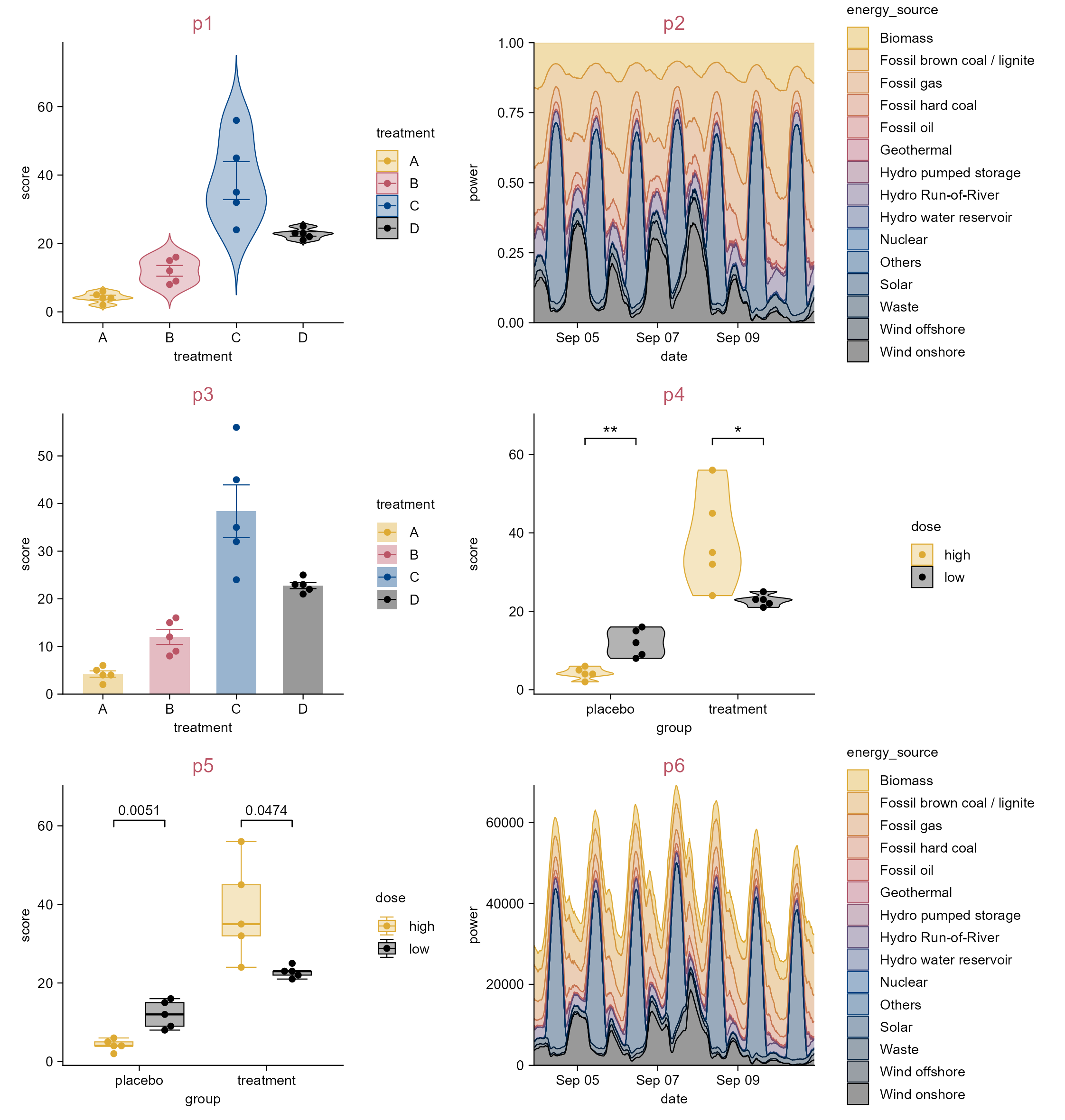

library(tidyplots)

p7 <- energy |> 
  tidyplot(y = energy, color = energy_source) |> 
  add_donut() |> 
  add_title(title = "p7")

df <- "https://tidyplots.org/data/correlation-matrix.csv" |>
  readr::read_csv(show_col_types =FALSE)

p8 <- df |> 
  tidyplot(x = x, y = y, color = correlation) |> 
  add_title(title = "p8") |> 
  add_heatmap() |> 
  sort_x_axis_levels(order_x) |> 
  sort_y_axis_levels(order_y) |> 
  remove_x_axis() |> remove_y_axis() |> remove_legend_title()

p9 <- spendings |> 
  tidyplot(x = category, y = amount, color = category) |> 
  add_title(title = "p9") |> 
  add_sum_bar(width = 0.05, alpha = 1) |> 
  add_sum_dot() |> 
  add_sum_value(accuracy = 1) |> 
  remove_legend() |> 
  adjust_x_axis(rotate_labels = 45)

p10 <- study |> 
  tidyplot(x = participant, y = score, color = group, dodge_width = 0) |> 
  add_title(title = "p10") |> 
  add_line(group = participant, color = "#bbbbbb") |> 
  add_data_points(size = 2.5)

p11 <- energy |> 
  tidyplot(y = energy, color = energy_source) |> 
  add_pie() |> 
  add_title(title = "p11")

p12 <- time_course |> 
  tidyplot(x = day, y = score, color = treatment) |> 
  add_title(title = "p12") |> 
  add_mean_line() |> 
  add_sem_ribbon()

patchwork::wrap_plots(p7, p8, p9, p10, p11, p12, ncol = 2) |> 
  save_plot("images/p7_p12.png",
    view_plot = FALSE, width = 200, height = 200) # width and height should be tailored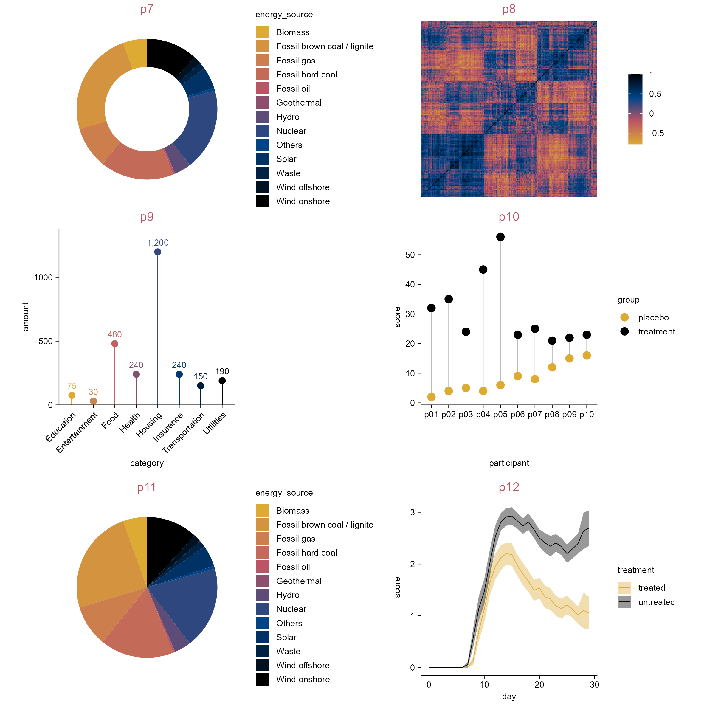

library(tidyplots)

p13 <- energy |> 
  tidyplot(x = year, y = energy, color = energy_type) |> 
  add_title(title = "p13") |> 
  add_barstack_absolute()

p14 <- climate |> 
  tidyplot(x = max_temperature) |> 
  add_title(title = "p14") |> 
  add_histogram()

p15 <- energy |> 
  tidyplot(x = year, y = energy, color = energy_type) |> 
  add_title(title = "p15") |> 
  add_barstack_relative()

p16 <- animals |> 
  tidyplot(x = weight, y = size) |> 
  add_title(title = "p16") |> 
  add_data_points(white_border = TRUE) |> 
  add_data_labels_repel(
    label = animal, 
    data = max_rows(weight, n = 3),
    color = "#000000",
    min.segment.length = 0)

df <- tibble::tibble(
  x = 1,
  y = 1,
  text = c("<span style='font-size:20pt;'>More (custom) plot types</span>
    <br><br><i>extented with ggplot2 (extentions) using <b>add()</b></i>."))

p17 <- df |> 
  tidyplot(x = x, y = y) |> 
  add_title(title = "p17") |> 
  add(ggtext::geom_richtext(
    ggplot2::aes(x = x, y = y, label = text), 
    data = df, 
    color = "#000000", 
    fill = "#ffcccc")) |> 
  add(ggplot2::theme_bw()) |> 
  adjust_size(width = 100)

design <- "AB
           CD
           EE"

(p13 + p14 + p15 + p16 + p17 + patchwork::plot_layout(design = design)) |> 
  save_plot("images/p13_p17.png",
    view_plot = FALSE, width = 165, height = 200) # width and height should be tailored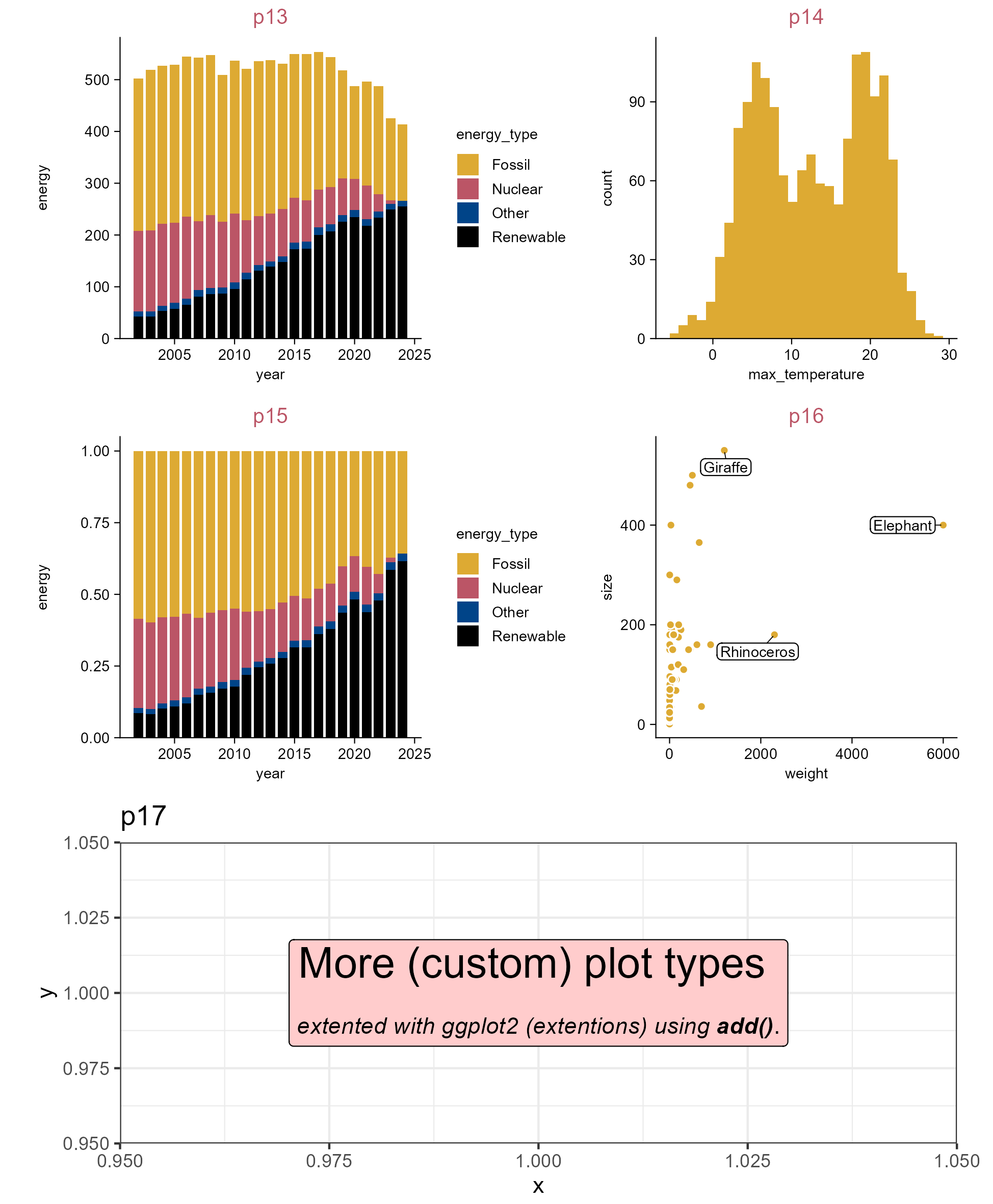

2.2 Anatomy of plot

study |> 
  tidyplot(x = group, y = score, color = dose) |> 
  add_mean_bar(alpha = 0.4) |> 
  add_sem_errorbar() |> 
  add_data_points_beeswarm(white_border = TRUE, size = 1.5) |> 
  add_title(title = "My study") |> 
  add_caption(caption = "Petterson et al.")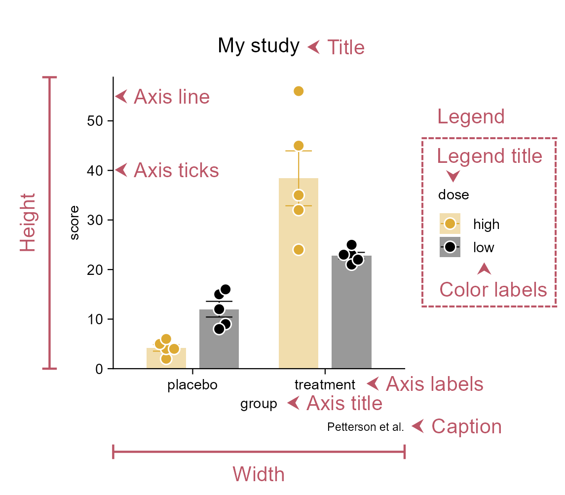

Note

All plots in tidyplots have absolute dimensions. By default this is 50 mm in width and 50 mm in height.