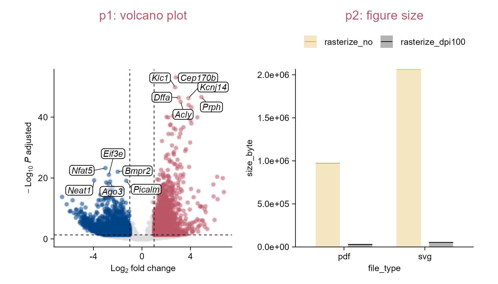
4  More plots

4.1 Violin plot

library(tidyplots)

# View top 10 rows of the columns used
study |> 
  dplyr::select(treatment, score) |> 
  dplyr::slice_head(n = 10)
# A tibble: 10 × 2
   treatment score
   <chr>     <dbl>
 1 A             2
 2 A             4
 3 A             5
 4 A             4
 5 A             6
 6 B             9
 7 B             8
 8 B            12
 9 B            15
10 B            16
p1 <- study |> 
  tidyplot(x = treatment, y = score, color = treatment) |> 
  add_data_points_beeswarm(white_border = TRUE) |> 
  add_title(title = "p1")

p2 <- p1 |> 
  adjust_title(title = "p2: violin without tail") |> 
  add_violin()

p3 <- p1 |> 
  adjust_title(title = "p3: violin with tail") |> 
  add_violin(trim = FALSE)

p4 <- p1 |> 
  adjust_title(title = "p4: violin with tail and quantiles") |> 
  add_violin(
    trim = FALSE, 
    quantile.linetype = "solid", 
    linewidth = 1)

p5 <- p2 |> 
  adjust_title(title = "p5: compare to 'A'") |> 
  add_test_asterisks(ref.group = "A", hide_info = TRUE)

p6 <- p3 |> 
  adjust_title(title = "p6: compare to 'A'") |> 
  add_test_pvalue(ref.group = "A", padding_top = 0.2, 
    bracket.nudge.y = 0.3, step.increase = 0.2, hide_info = TRUE)

Violin plot.

4.2 (Rasterize) correlation heatmap

library(tidyplots)

df <- "https://tidyplots.org/data/correlation-matrix.csv" |> 
  readr::read_csv(show_col_types = FALSE)
df |> dim()
[1] 202500      5
# View top 10 rows of the columns used
df |> dplyr::select(x, y, correlation) |> 
  dplyr::slice_head(n = 10)
# A tibble: 10 × 3
   x       y       correlation
   <chr>   <chr>         <dbl>
 1 YAL022C YAL022C      1     
 2 YAL022C YAL040C      0.505 
 3 YAL022C YAL053W      0.0730
 4 YAL022C YAL067C     -0.244 
 5 YAL022C YAR003W      0.0282
 6 YAL022C YAR007C     -0.197 
 7 YAL022C YAR008W     -0.0395
 8 YAL022C YAR018C      0.692 
 9 YAL022C YBL002W     -0.0289
10 YAL022C YBL003C     -0.125 
# Define a new color scheme
new_colors <- c("#000000", "#994455", "#ee99aa", "#eecc66")

p0 <- df |> 
  tidyplot(x = x, y = y, color = correlation) |>    
  remove_legend_title() |> 
  adjust_colors(new_colors = new_colors) |> 
  adjust_theme_details(legend.key.height = ggplot2::unit(1, "null"),
    legend.margin = ggplot2::margin_part(t = 0, b = 0)) |> 
  add_caption("Data source: Mol Biol Cell. 1998. PMID: 9843569")

# Save vector images without rasterization
p0 |> 
  add_heatmap() |> 
  sort_x_axis_levels(order_x) |> sort_y_axis_levels(order_y) |> 
  remove_x_axis() |> remove_y_axis() |> 
  save_plot("images/rasterize_correlation_no.pdf", view_plot = FALSE) |> 
  save_plot("images/rasterize_correlation_no.svg", view_plot = FALSE)

# Save vector images with rasterization (dpi = 100)
p0 |> 
  add_heatmap(rasterize = TRUE, rasterize_dpi = 100) |> 
  sort_x_axis_levels(order_x) |> sort_y_axis_levels(order_y) |> 
  remove_x_axis() |> remove_y_axis() |> 
  save_plot("images/rasterize_correlation_yes_dpi100.pdf", view_plot = FALSE) |> 
  save_plot("images/rasterize_correlation_yes_dpi100.svg", view_plot = FALSE)

List the figures saved:

images
├── rasterize_correlation_no.pdf
├── rasterize_correlation_no.svg
├── rasterize_correlation_yes_dpi100.pdf
└── rasterize_correlation_yes_dpi100.svg

Rasterize correlation heatmap selectively.

4.3 Heatmap (z-score)

Tip

This is expecially useful when you want to focus on the dynamics within rows or columns.

library(tidyplots)

# View top 10 rows of the columns used
climate |> 
  dplyr::select(month, year, max_temperature) |> 
  dplyr::slice_head(n = 10)
# A tibble: 10 × 3
   month  year max_temperature
   <chr> <dbl>           <dbl>
 1 01     1891           -1.49
 2 02     1891            3.37
 3 03     1891            5.05
 4 04     1891            8.34
 5 05     1891           16.2 
 6 06     1891           18.2 
 7 07     1891           20.5 
 8 08     1891           18.2 
 9 09     1891           18.3 
10 10     1891           14.2 
# Plot
p1 <- climate |> 
  tidyplot(
    x = month, 
    y = year, 
    color = max_temperature) |> 
  adjust_colors(new_colors = c(
    "#ddaa33", 
    "#ffffff", 
    "#bb5566")) |>
  add_title("p1")

p2 <- p1 |> 
  adjust_title("p2: max temperature") |> 
  add_heatmap() 

p3 <- p1 |> 
  add_heatmap(scale = "row") |> 
  adjust_colors(new_colors = c(
    "#ddaa33", 
    "#ffffff", 
    "#bb5566")) |> 
  adjust_title("p3: row z-score")

p4 <- p2 |> 
  sort_x_axis_levels(max_temperature) |>
  adjust_title(paste(
    "p4: max_temperature", 
    "sort x axis levels", 
    sep = "\n"))

Heatmap_z-scores.

4.4 (Rasterize) volcano plot

library(tidyplots)

df <- 
  "https://tidyplots.org/data/differential-expression-analysis.csv" |> 
  readr::read_csv(show_col_types = FALSE) |> 
  dplyr::mutate(
    neg_log10_padj = -log10(padj),
    direction = dplyr::if_else(log2FoldChange > 0, "up", "down", "NA"),
    candidate = abs(log2FoldChange) >= 1 & padj < 0.05)
df |> dim()
[1] 43629    17
# View top 10 rows of the columns used
df |> 
  dplyr::select(
    log2FoldChange, neg_log10_padj, candidate, 
    direction, padj, external_gene_name) |> 
  dplyr::slice_head(n = 10)
# A tibble: 10 × 6
   log2FoldChange neg_log10_padj candidate direction     padj external_gene_name
            <dbl>          <dbl> <lgl>     <chr>        <dbl> <chr>             
 1         -0.989         0.642  FALSE     down       2.28e-1 Gnai3             
 2         NA            NA      NA        <NA>      NA       Pbsn              
 3          0.342         0.0913 FALSE     up         8.10e-1 Cdc45             
 4          0.865         0.322  FALSE     up         4.77e-1 H19               
 5         -0.998         0.284  FALSE     down       5.20e-1 Scml2             
 6         -1.47          0.458  FALSE     down       3.48e-1 Apoh              
 7         -0.696         0.539  FALSE     down       2.89e-1 Narf              
 8         -2.52          4.02   TRUE      down       9.52e-5 Cav2              
 9         -1.26          2.04   TRUE      down       9.06e-3 Klf6              
10         -0.648         0.317  FALSE     down       4.82e-1 Scmh1             
p0 <- df |> 
  tidyplot(x = log2FoldChange, y = neg_log10_padj) |> 
  add_data_labels_repel(
    data = min_rows(padj, 6, by = direction), 
    label = external_gene_name, 
    color = "#000000", 
    min.segment.length = 0, 
    background = TRUE, 
    fontface = "italic") |> 
  adjust_x_axis_title("$Log[2]~fold~change$") |> 
  adjust_y_axis("$-Log[10]~italic(P)~adjusted$")

# Save vector images without rasterization
p0 |> 
  add_data_points(data = filter_rows(!candidate), color = "#dddddd") |> 
  add_data_points(
    data = filter_rows(candidate, direction == "up"), 
    color = "#bb5566", alpha = 0.5) |> 
  add_data_points(
    data = filter_rows(candidate, direction == "down"), 
    color = "#004488", alpha = 0.5) |>   
  add_reference_lines(x = c(-1, 1), y = -log10(0.05)) |> 
  save_plot("images/rasterize_volcano_no.pdf", view_plot = FALSE) |> 
  save_plot("images/rasterize_volcano_no.svg", view_plot = FALSE)

# Save vector images with rasterization (dpi = 100)
p0 |>   
  add_data_points(data = filter_rows(!candidate), color = "#dddddd", 
  rasterize = TRUE, rasterize_dpi = 100) |> 
  add_data_points(
    data = filter_rows(candidate, direction == "up"), color = "#bb5566", 
    alpha = 0.5, rasterize = TRUE, rasterize_dpi = 100) |> 
  add_data_points(
    data = filter_rows(candidate, direction == "down"), color = "#004488", 
    alpha = 0.5, rasterize = TRUE, rasterize_dpi = 100) |>   
  add_reference_lines(x = c(-1, 1), y = -log10(0.05)) |> 
  save_plot("images/rasterize_volcano_yes_dpi100.pdf", view_plot = FALSE) |> 
  save_plot("images/rasterize_volcano_yes_dpi100.svg", view_plot = FALSE)

List the figures saved:

images
├── rasterize_correlation_no.pdf
├── rasterize_correlation_no.svg
├── rasterize_correlation_yes_dpi100.pdf
└── rasterize_correlation_yes_dpi100.svg

Rasterize volcano plot selectively.

4.5 Lollipop plot

library(tidyplots)

# View top 10 rows of the columns used
spendings |> 
  dplyr::select(amount, category) |> 
  dplyr::slice_head(n = 10)
# A tibble: 10 × 2
   amount category      
    <dbl> <chr>         
 1    100 Food          
 2     40 Transportation
 3   1200 Housing       
 4     80 Utilities     
 5     75 Education     
 6    200 Insurance     
 7     60 Food          
 8     50 Utilities     
 9     90 Food          
10     40 Transportation
# Plot
p1 <- spendings |> 
  tidyplot(
    x = amount, 
    y = category, 
    color = category) |> 
  add_sum_bar(
    width = 0.8, 
    alpha = 0.2) |> 
  add_sum_dot() |> 
  add_title("p1: wide bars") |> 
  remove_legend()

p2 <- spendings |> 
  tidyplot(
    x = amount, 
    y = category, 
    color = category) |> 
  add_sum_bar(
    width = 0.05, 
    alpha = 1) |> 
  add_sum_dot() |> 
  add_title("p2: lollipop plot") |> 
  remove_legend()

Lollipop plot.
Tip

In essence, lollipop plot is generated via narrowing down bar width.

4.6 Dumbbell plot

library(tidyplots)

# View top 10 rows of the columns used
study |> 
  dplyr::select(participant, score, group) |> 
  dplyr::slice_head(n = 10)
# A tibble: 10 × 3
   participant score group  
   <chr>       <dbl> <chr>  
 1 p01             2 placebo
 2 p02             4 placebo
 3 p03             5 placebo
 4 p04             4 placebo
 5 p05             6 placebo
 6 p06             9 placebo
 7 p07             8 placebo
 8 p08            12 placebo
 9 p09            15 placebo
10 p10            16 placebo
# Plot
p1 <- study |> 
  tidyplot(
    x = participant, 
    y = score, 
    color = group) |> 
  add_data_points(size = 2.5) |> 
  add_title(title = "p1")

p2 <- p1 |> 
  adjust_title(title = "p2: add 'group'-based lines") |>  
  add_line(color = "#bbbbbb") |> 
  remove_legend()

p3 <- p1 |> 
  adjust_title(title = "p3: add 'participant'-based lines") |> 
  add_line(
    group = participant, 
    color = "#bbbbbb") |>   
  remove_legend()

p4 <- study |> 
  tidyplot(
    x = participant, 
    y = score, 
    color = group, 
    dodge_width = 0) |> 
  add_title(title = "p4: dumbbell plot") |> 
  add_line(
    group = participant, 
    color = "#bbbbbb") |> 
  add_data_points(size = 2.5) |> 
  remove_legend()

Dumbbell plot.

4.7 Pie and donut plots

library(tidyplots)

# View top 10 rows of the columns used
energy |> 
  dplyr::select(energy, energy_source) |> 
  dplyr::slice_head(n = 10)
# A tibble: 10 × 2
    energy energy_source              
     <dbl> <fct>                      
 1   3.72  Biomass                    
 2 141.    Fossil brown coal / lignite
 3  40.0   Fossil gas                 
 4 111.    Fossil hard coal           
 5   1.76  Fossil oil                 
 6   0     Geothermal                 
 7  23.4   Hydro                      
 8 156.    Nuclear                    
 9   6.31  Others                     
10   0.196 Solar                      
# Plot
p0 <- energy |> 
  tidyplot(
    y = energy, 
    color = energy_type)

p1 <- p0 |> 
  add_pie() |> 
  add_title(title = "p1: pie")

p2 <- p0 |>  
  add_donut() |> 
  add_title(title = "p2: donut")

p3 <- p0 |> 
  add_donut(alpha = 0.5) |> 
  add_title(title = paste("p3: donut", "alpha = 0.5", sep = "\n"))

p4 <- p0 |> 
  add_donut(reverse = TRUE) |> 
  add_title(title = paste("p4: donut", "reverse = TRUE", sep = "\n"))

p5 <- p0 |> 
  add_donut(width = 2) |> 
  add_title(title = paste("p5: donut", "width = 2", sep = "\n"))

p6 <- p0 |> 
  add_donut(width = 4) |> 
  add_title(title = paste("p6: donut", "width = 4", sep = "\n"))

Donut and pie plots.

4.8 Stacked bar plot

library(tidyplots)

# View top 10 rows of the columns used
energy |> 
  dplyr::select(year, energy, energy_type) |> 
  dplyr::slice_head(n = 10)
# A tibble: 10 × 3
    year  energy energy_type
   <dbl>   <dbl> <fct>      
 1  2002   3.72  Renewable  
 2  2002 141.    Fossil     
 3  2002  40.0   Fossil     
 4  2002 111.    Fossil     
 5  2002   1.76  Fossil     
 6  2002   0     Renewable  
 7  2002  23.4   Renewable  
 8  2002 156.    Nuclear    
 9  2002   6.31  Other      
10  2002   0.196 Renewable  
# Plot
p1 <- energy |> 
  tidyplot(y = energy, color = energy_type) |> 
  add_title(title = "p1: absolute") |> 
  add_barstack_absolute()

p2 <- energy |> 
  tidyplot(y = energy, color = energy_type) |> 
  add_title(title = "p2: relative") |> 
  add_barstack_relative() |> 
  remove_legend()

p3 <- energy |> 
  tidyplot(x = year, y = energy, color = energy_type) |> 
  add_title(title = "p3: absolute (year-based)") |> 
  add_barstack_absolute() |>
  remove_legend()  

p4 <- energy |> 
  tidyplot(x = year, y = energy, color = energy_type) |> 
  add_title(title = "p4: relative (year-based)") |> 
  add_barstack_relative() |>
  remove_legend() 

p5 <- energy |> 
  tidyplot(x = energy, y = year, color = energy_type) |> 
  add_title(title = "p5: p4 horizontal") |> 
  add_barstack_relative(orientation = "y") |> 
  remove_legend()

Stacked bar plot.

4.9 Histogram

library(tidyplots)

# View top 10 rows of the columns used
climate |> 
  dplyr::select(max_temperature, month) |> 
  dplyr::slice_head(n = 10)
# A tibble: 10 × 2
   max_temperature month
             <dbl> <chr>
 1           -1.49 01   
 2            3.37 02   
 3            5.05 03   
 4            8.34 04   
 5           16.2  05   
 6           18.2  06   
 7           20.5  07   
 8           18.2  08   
 9           18.3  09   
10           14.2  10   
# Plot
p0 <- climate |> 
  tidyplot(x = max_temperature)

p1 <- p0 |> 
  add_title(title = "p1: bins = 30 (default)") |> 
  add_histogram(color = "#bb5566")

p2 <- p0 |> 
  add_title(title = paste("p2: bins = 60", "density", sep = "\n")) |> 
  add_histogram(bins = 60, mapping = ggplot2::aes(y = ggplot2::after_stat(density)))

p3 <- p0 |>
  add_histogram(color = rep(c("#ddaa33", "#004488"), length.out = 30)) |> 
  adjust_title(title = "p3: bars and lines") |> 
  add(ggplot2::geom_freqpoly(bins = 30, color = "#000000"))

p4 <- climate |> 
  tidyplot(y = max_temperature) |>   
  add_title(title = "p4: bars in y axis") |> 
  add_histogram(color = rep(c("#ee99aa", "#994455"), each  = 15))

p5 <- climate |> 
  dplyr::filter(month %in% c("01", "03", "06")) |> 
  tidyplot(x = max_temperature, color = month) |> 
  add_title(title = "p5: month-based") |> 
  add_histogram(alpha = 0.5)

p6 <- climate |> 
  dplyr::filter(month %in% c("01", "03", "06")) |> 
  tidyplot(x = max_temperature, color = month) |> 
  add_title(title = "p6: density_smooth") |> 
  add(ggplot2::geom_density(ggplot2::aes(color = month), 
    position = ggplot2::position_identity(), alpha = 0.2))

Histogram.