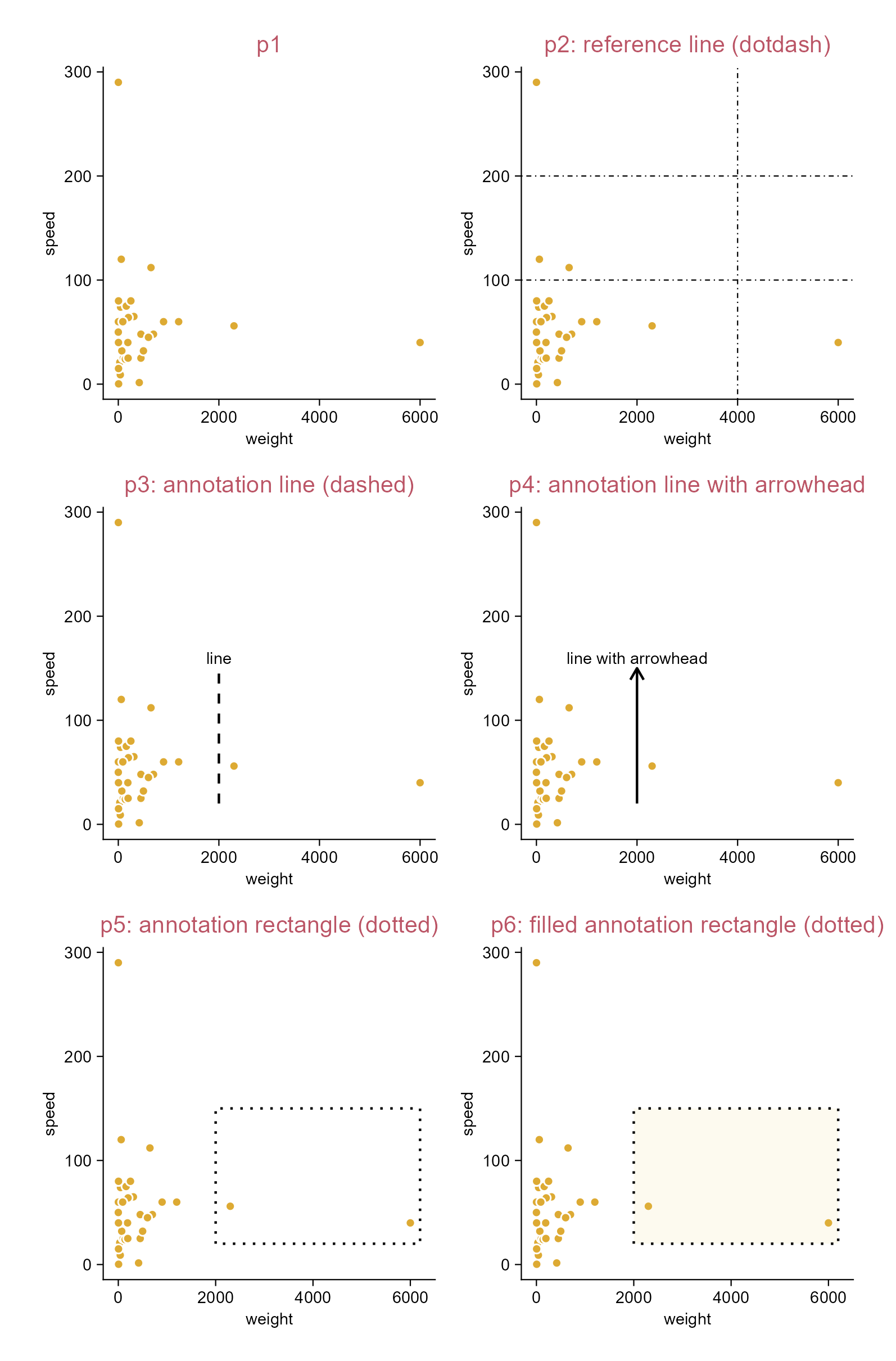
p1 <- animals |>tidyplot(x = weight, y = speed) |>add_data_points(white_border =TRUE) |>add_title(title ="p1") p2 <- p1 |>adjust_title(title ="p2: reference line (dotdash)") |>add_reference_lines(x =4000, y =c(100, 200), linetype ="dotdash")p3 <- p1 |>adjust_title(title ="p3: annotation line (dashed)") |>add_annotation_line(x =2000, xend =2000, y =20, yend =150, linetype ="dashed") |>add_annotation_text(text ="line", x =2000, y =160)p4 <- p1 |>adjust_title(title ="p4: annotation line with arrowhead") |>add_annotation_line(x =2000, xend =2000, y =20, yend =150,arrow = grid::arrow(length = grid::unit(2, "mm"))) |>add_annotation_text(text ="line with arrowhead", x =2000, y =160)p5 <- p1 |>adjust_title(title ="p5: annotation rectangle (dotted)") |>add_annotation_rectangle(xmin =2000, xmax =6200, ymin =20, ymax =150, linetype ="dotted", color ="#000000", fill =NA)p6 <- p1 |>adjust_title(title ="p6: filled annotation rectangle (dotted)") |>add_annotation_rectangle(xmin =2000, xmax =6200, ymin =20, ymax =150, linetype ="dotted", color ="#000000", fill ="#eecc66")
Add reference lines or rectangle.
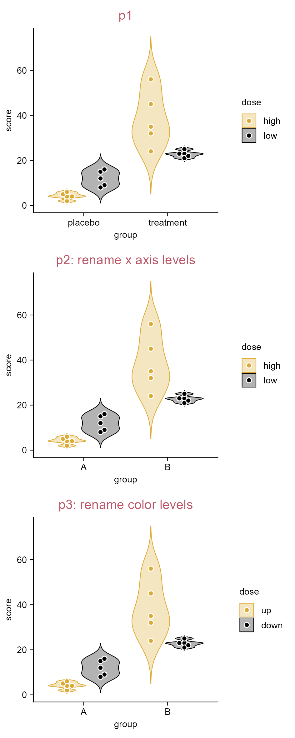
3.9 Rename axis levels (e.g. violin plot)
library(tidyplots)# View the top 10 rows of the columns usedstudy |> dplyr::select(group, score, dose) |> dplyr::slice_head(n =10)
# A tibble: 10 × 3
group score dose
<chr> <dbl> <chr>
1 placebo 2 high
2 placebo 4 high
3 placebo 5 high
4 placebo 4 high
5 placebo 6 high
6 placebo 9 low
7 placebo 8 low
8 placebo 12 low
9 placebo 15 low
10 placebo 16 low
# Plotp1 <- study |>tidyplot(x = group, y = score, color = dose) |>add_violin(trim =FALSE) |>add_data_points_beeswarm(white_border =TRUE) |>add_title(title ="p1")p2 <- p1 |>adjust_title(title ="p2: rename x axis levels") |>rename_x_axis_levels(new_names =c("placebo"="A", "treatment"="B"))p3 <- p2 |>adjust_title(title ="p3: rename color levels") |>rename_color_levels(new_names =c("high"="up", "low"="down"))
Rename axis levels.
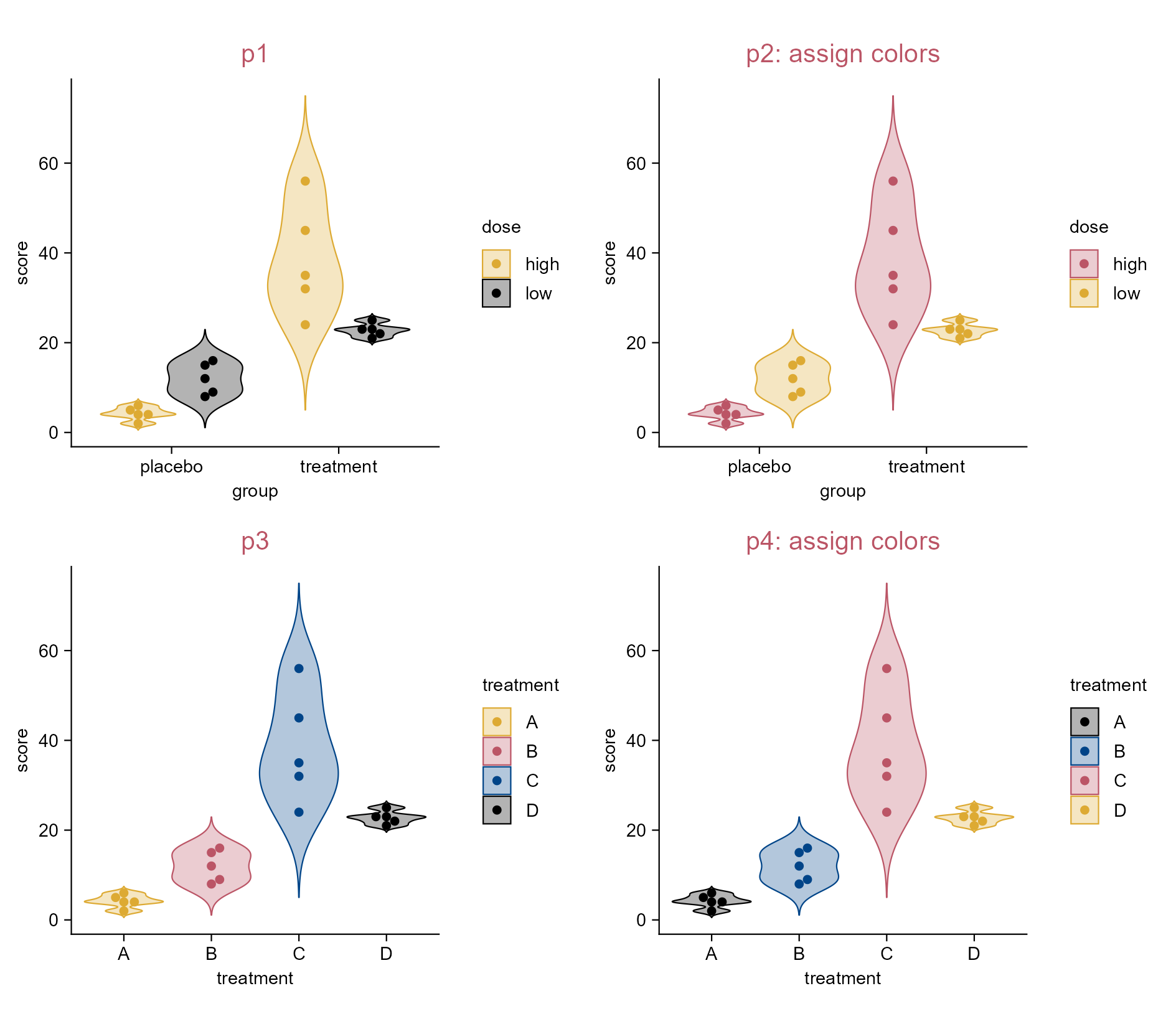
3.10 Assign colors (e.g. violin plot)
library(tidyplots)# View top 10 rows of the columns usedstudy |> dplyr::select(group, score, dose) |> dplyr::slice_head(n =10)
# A tibble: 10 × 3
group score dose
<chr> <dbl> <chr>
1 placebo 2 high
2 placebo 4 high
3 placebo 5 high
4 placebo 4 high
5 placebo 6 high
6 placebo 9 low
7 placebo 8 low
8 placebo 12 low
9 placebo 15 low
10 placebo 16 low
p1 <- study |>tidyplot(x = group, y = score, color = dose) |>add_violin(trim =FALSE) |>add_data_points_beeswarm() |>add_title(title ="p1") p2 <- p1 |>adjust_title(title ="p2: assign colors") |>adjust_colors(new_colors =c("high"="#bb5566", "low"="#ddaa33"))p3 <- study |>tidyplot(x = treatment, y = score, color = treatment) |>add_violin(trim =FALSE) |>add_data_points_beeswarm() |>add_title(title ="p3")p4 <- p3 |>adjust_title(title ="p4: assign colors") |>adjust_colors(new_colors =c("A"="#000000", "B"="#004488","C"="#bb5566", "D"="#ddaa33"))
Assign colors.
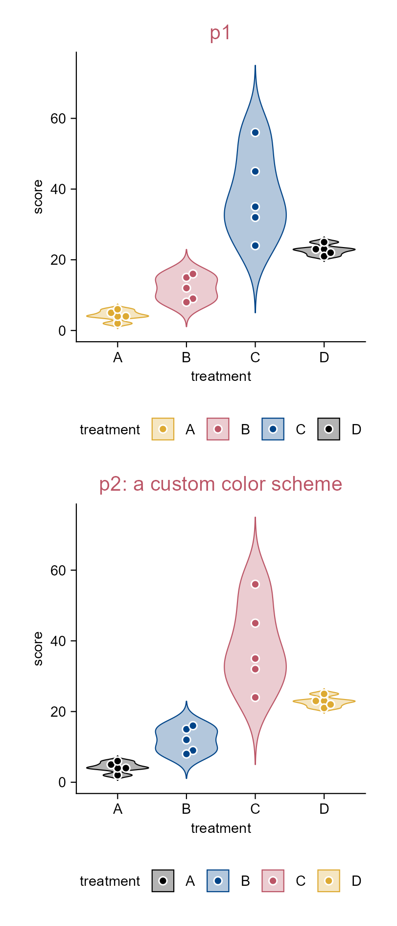
3.11 Define a custom color scheme (e.g. violin plot)
library(tidyplots)# Define a custom color schemehigh_contrast_qualitative_colour <-new_color_scheme(c("#000000", "#004488", "#bb5566", "#ddaa33"), name ="high_contrast_qualitative_colour")# View top 10 rows of the columns usedstudy |> dplyr::select(treatment, score) |> dplyr::slice_head(n =10)
# A tibble: 10 × 2
   treatment score
   <chr>     <dbl>
 1 A             2
 2 A             4
 3 A             5
 4 A             4
 5 A             6
 6 B             9
 7 B             8
 8 B            12
 9 B            15
10 B            16
# Plotp1 <- study |>tidyplot(x = treatment, y = score, color = treatment) |>add_violin(trim =FALSE) |>add_data_points_beeswarm(white_border =TRUE) |>adjust_legend_position(position ="bottom") |>add_title(title ="p1")p2 <- p1 |>adjust_title(title ="p2: a custom color scheme") |>adjust_colors(new_colors = high_contrast_qualitative_colour)
Define a custom color scheme.
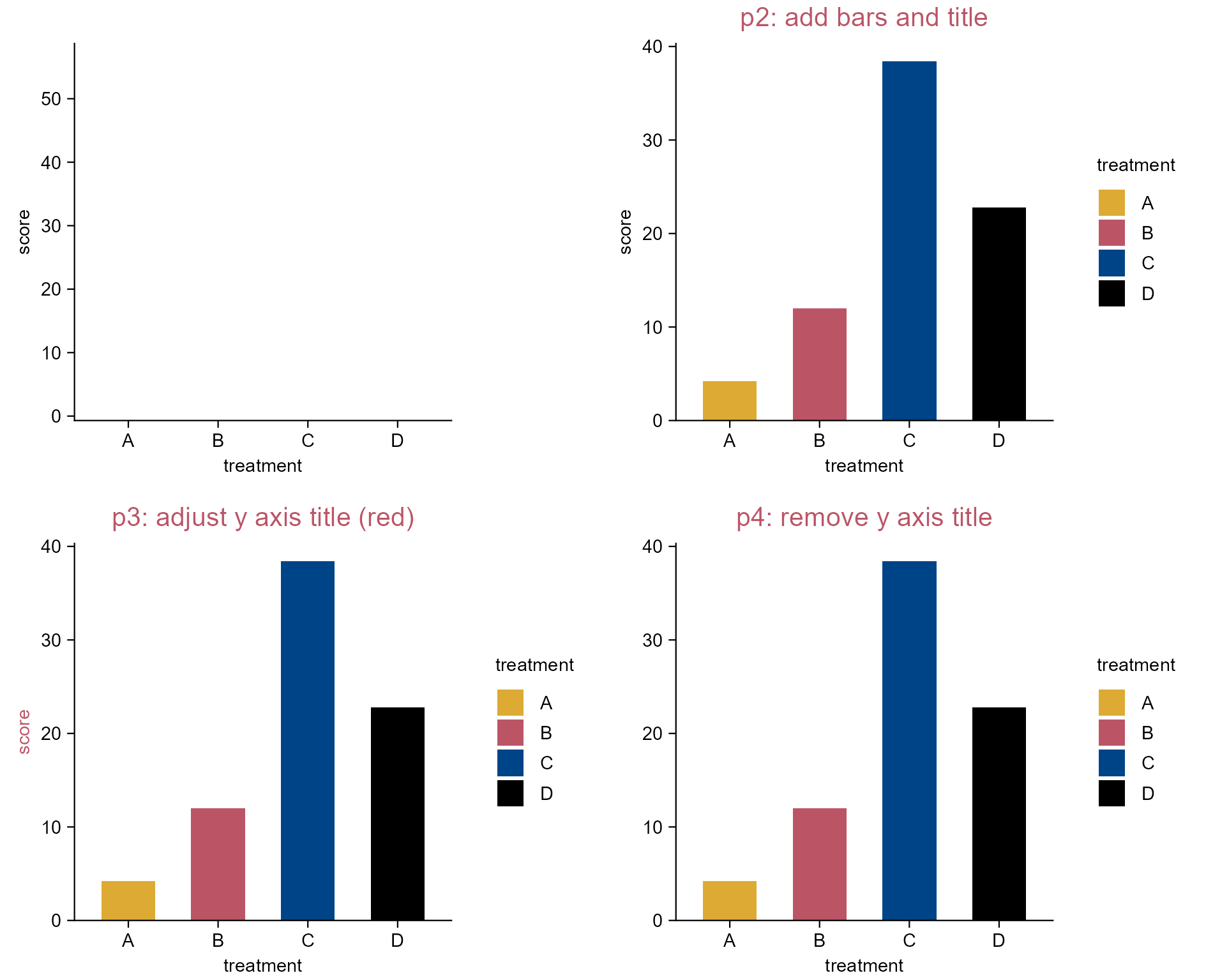
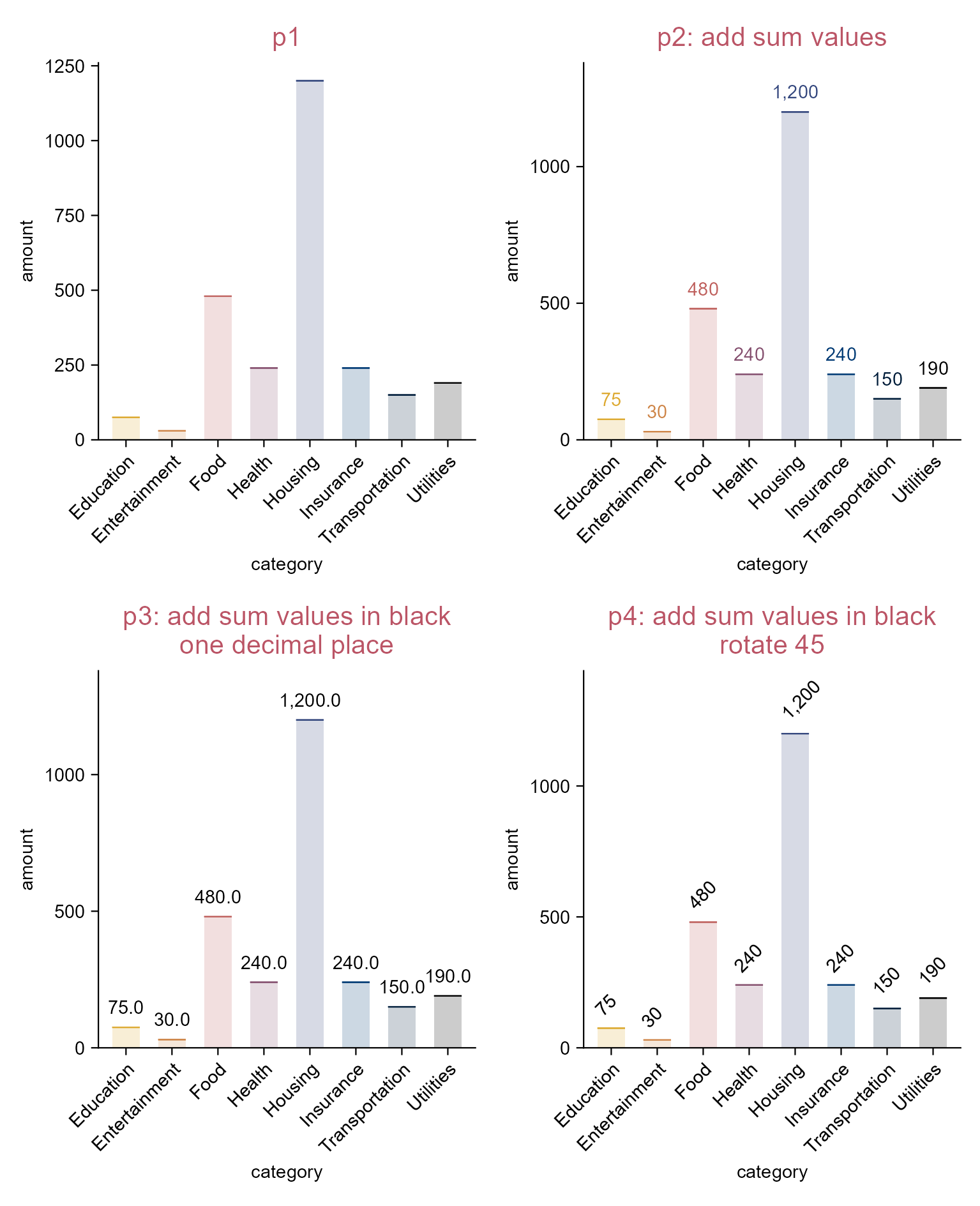
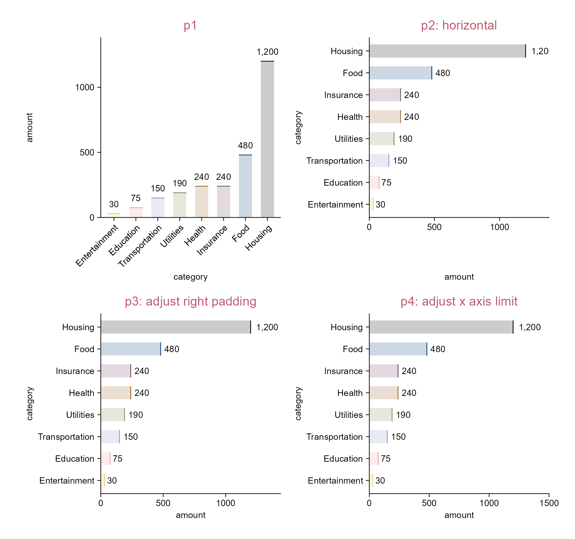
3.12 Add sum values (e.g. bar plot)
library(tidyplots)# View top 10 rows of the columns usedspendings |> dplyr::select(category, amount) |> dplyr::slice_head(n =10)
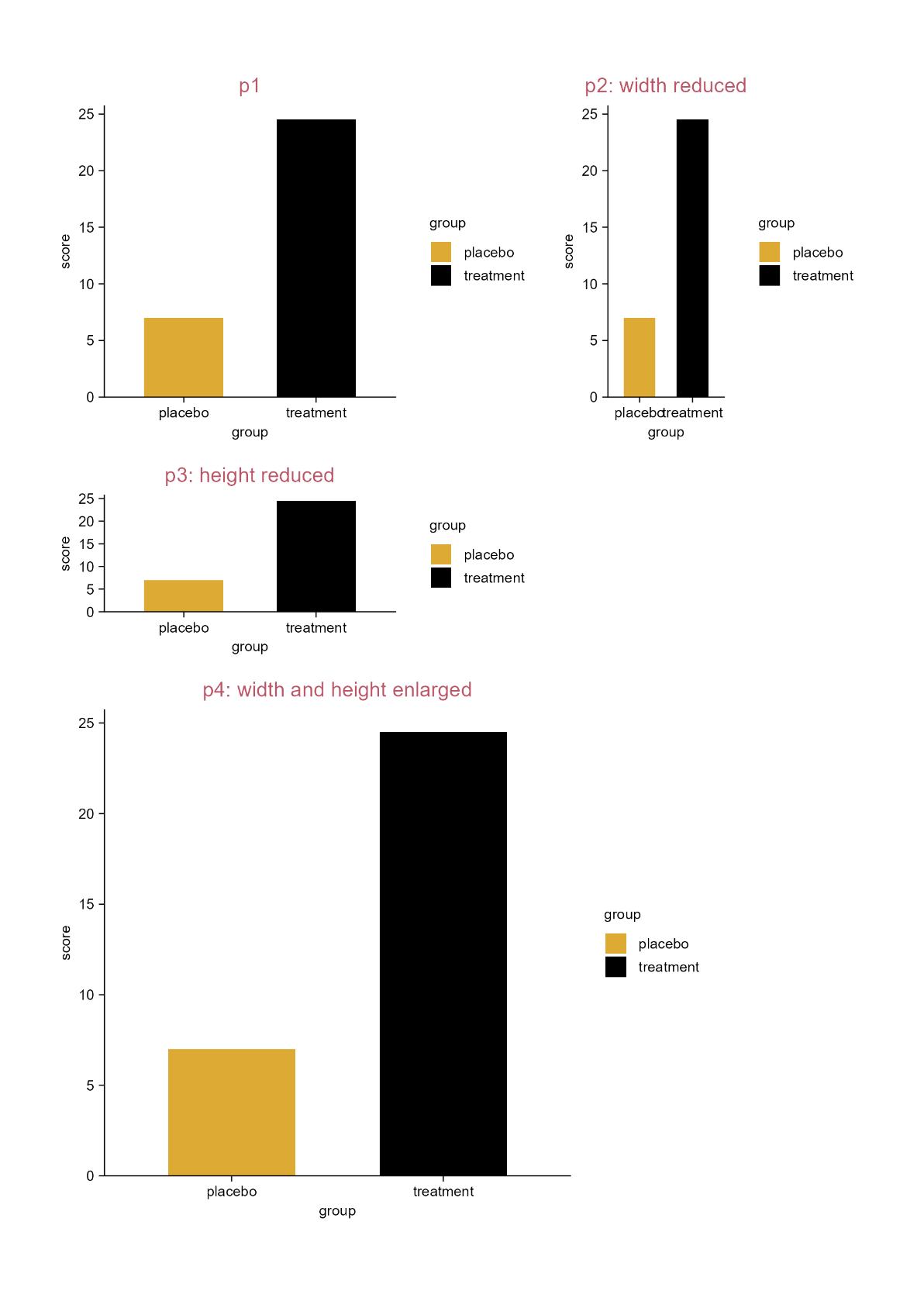
The sum value of Housing in p2 is clipped (the actual value should be 1,200).
One way to solve this is via p3 (i.e. piping with adjust_padding(right = 0.2)).
The second way is via p4 (i.e. piping with adjust_x_axis(limits = c(0, 1500)).
The third way is to pipe with remove_clipping() if you install a specific commit (on 2026-04-01), i.e. pak("jbengler/tidyplots@4a08bfe") via the pak package, or use a later version.
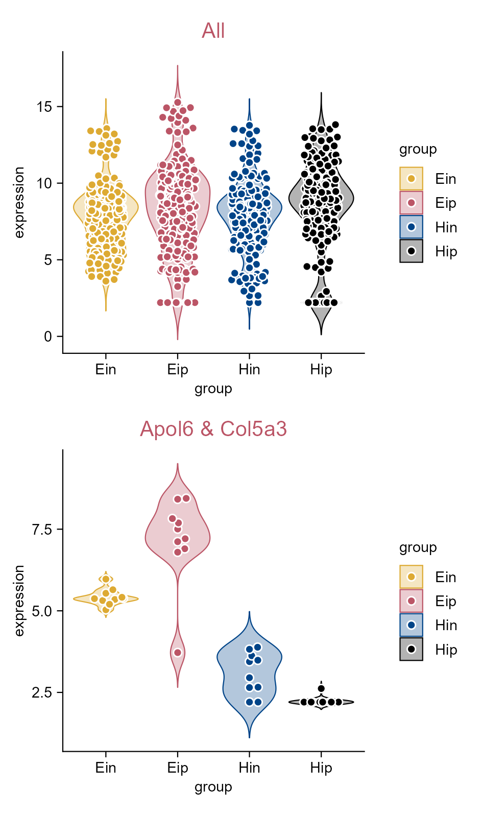
3.17 Preview a subset of dataset (e.g. violin plot)
library(tidyplots)# View top 10 rows of the columns usedgene_expression |> dplyr::select(group, expression, external_gene_name) |> dplyr::slice_head(n =10)
# A tibble: 10 × 3
group expression external_gene_name
<chr> <dbl> <chr>
1 Hin 2.20 Apol6
2 Hin 2.20 Apol6
3 Hin 2.66 Apol6
4 Hin 2.65 Apol6
5 Hin 3.44 Apol6
6 Ein 5.03 Apol6
7 Ein 5.31 Apol6
8 Ein 5.37 Apol6
9 Ein 5.54 Apol6
10 Ein 5.65 Apol6
library(tidyplots)# View top 10 rows of the columns usedstudy |> dplyr::select(group, score, dose) |> dplyr::slice_head(n =10)
# A tibble: 10 × 3
group score dose
<chr> <dbl> <chr>
1 placebo 2 high
2 placebo 4 high
3 placebo 5 high
4 placebo 4 high
5 placebo 6 high
6 placebo 9 low
7 placebo 8 low
8 placebo 12 low
9 placebo 15 low
10 placebo 16 low
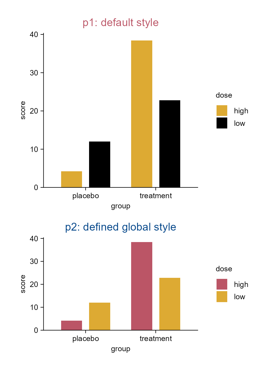
# eval: false# Define a global stylemy_style <-function(x) { x |>adjust_colors(new_colors =c("#bb5566", "#ddaa33")) |>adjust_size(width =50, height =30, unit ="mm") |>adjust_title(fontsize =10, color ="#004488")}# Plotp1 <- study |>tidyplot(x = group, y = score, color = dose) |>add_mean_bar() |>adjust_size() |>add_title("p1: default style")# Set global optionstidyplots_options(my_style = my_style)# Plotp2 <- study |>tidyplot(x = group, y = score, color = dose) |>add_mean_bar() |>add_title("p2: defined global style")
Set a global default style.
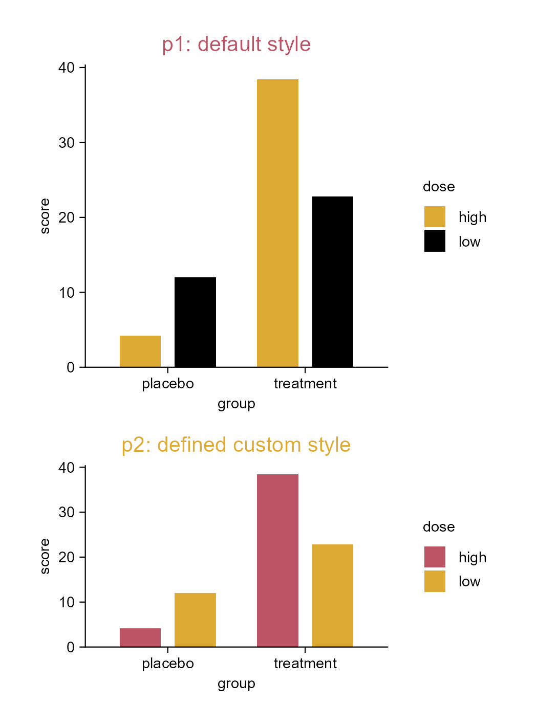
3.19 Set a custom style to reuse (e.g. bar plot)
library(tidyplots)# View top 10 rows of the columns usedstudy |> dplyr::select(group, score, dose) |> dplyr::slice_head(n =10)
# A tibble: 10 × 3
group score dose
<chr> <dbl> <chr>
1 placebo 2 high
2 placebo 4 high
3 placebo 5 high
4 placebo 4 high
5 placebo 6 high
6 placebo 9 low
7 placebo 8 low
8 placebo 12 low
9 placebo 15 low
10 placebo 16 low
# Define a stylemy_style <-function(x) { x |>adjust_colors(new_colors =c("#bb5566", "#ddaa33")) |>adjust_size(width =50, height =30, unit ="mm") |>adjust_title(fontsize =10, color ="#ddaa33")}p1 <- study |>tidyplot(x = group, y = score, color = dose) |>add_mean_bar() |>adjust_size() |>add_title("p1: default style")p2 <- study |>tidyplot(x = group, y = score, color = dose) |>add_mean_bar() |>add_title("p2: defined custom style") |>my_style()
Set a custom style to reuse.
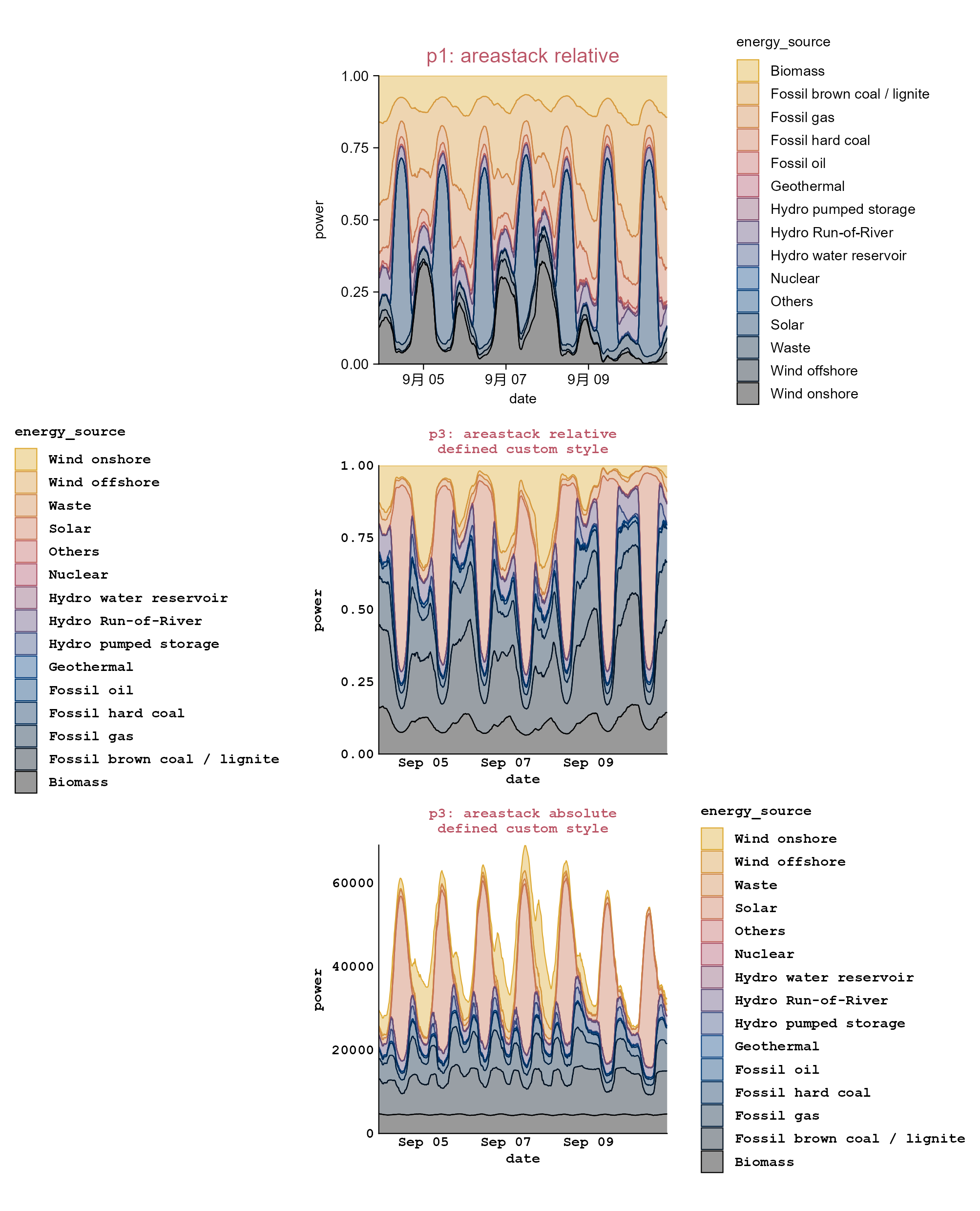
3.20 Set a custom style to reuse (e.g. areastack plot)
library(tidyplots)# View top 10 rows of the columns usedenergy_week |> dplyr::select(date, power, energy_source) |> dplyr::slice_head(n =10)
Please note the Chinese character “月” on the x-axis of p1, as the code was run on an x86_64-w64-mingw32/x64 platform with the locale set to Chinese (Simplified)_China.utf8.
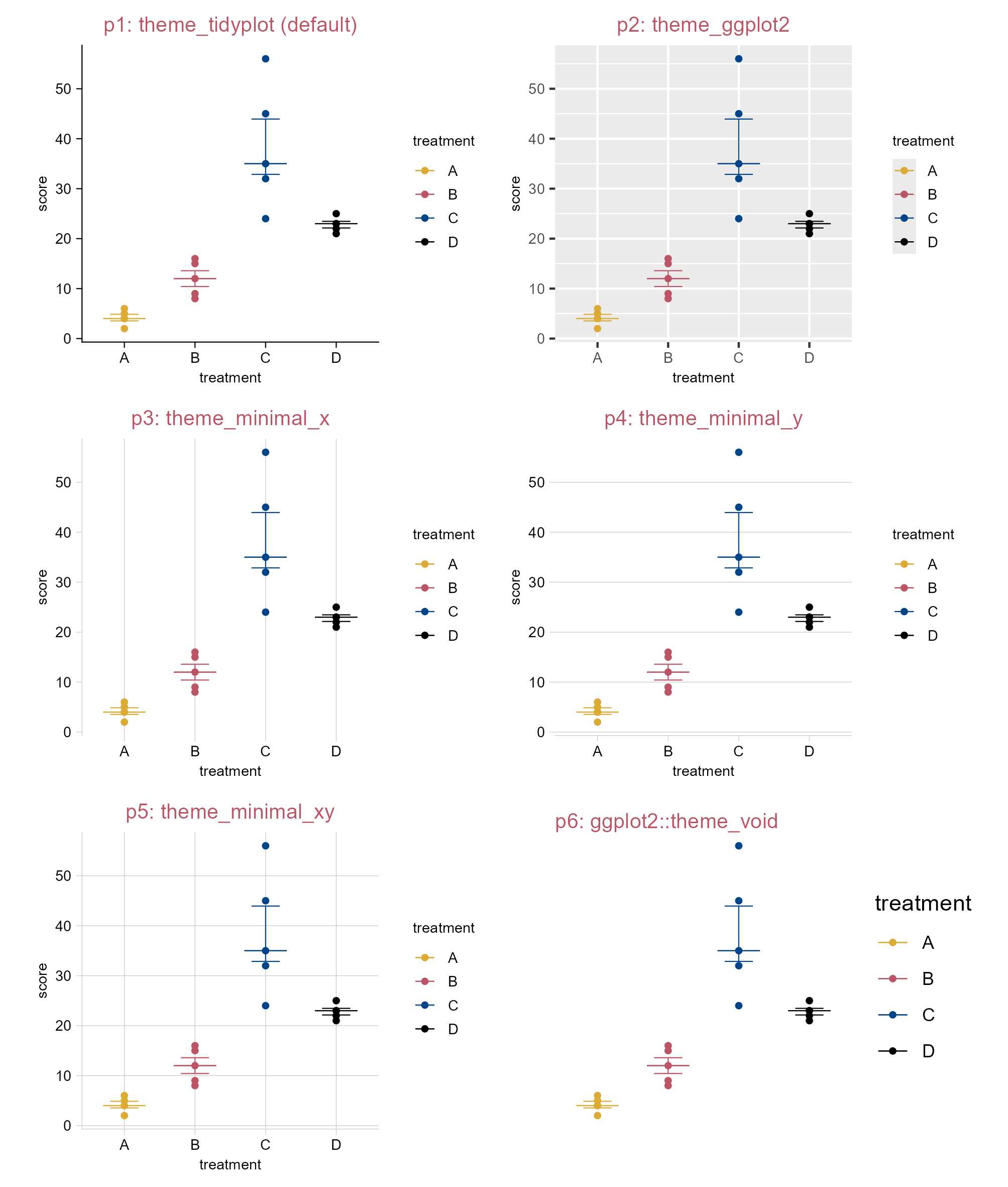
3.21 Plot paper and ink colors (e.g. bar plot)
library(tidyplots)# View top 10 rows of the columns usedstudy |> dplyr::select(treatment, score) |> dplyr::slice_head(n =10)
# A tibble: 10 × 2
   treatment score
   <chr>     <dbl>
 1 A             2
 2 A             4
 3 A             5
 4 A             4
 5 A             6
 6 B             9
 7 B             8
 8 B            12
 9 B            15
10 B            16
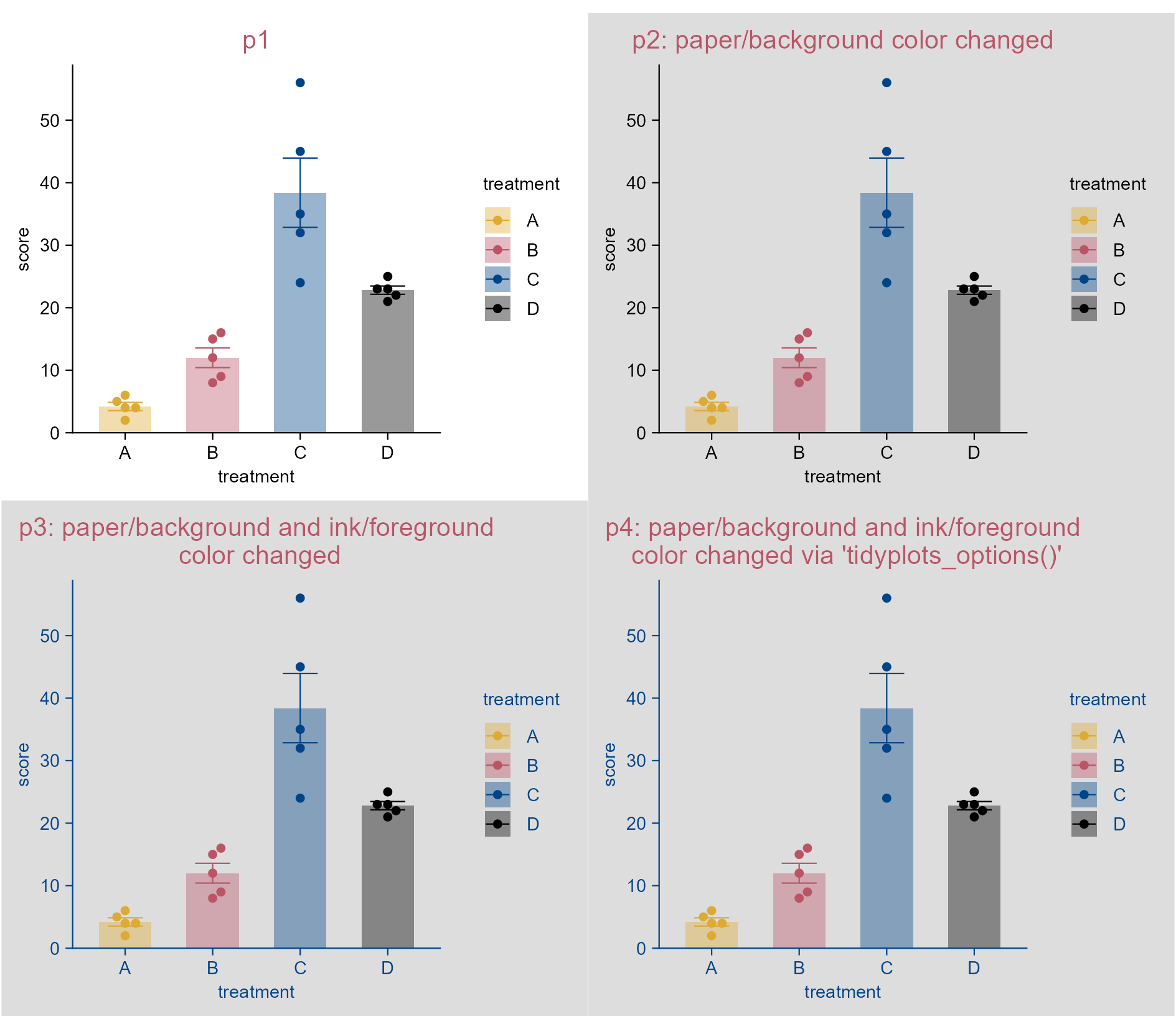
# Define a style to reusemy_style <-function(x) { x |>add_mean_bar(alpha =0.4) |>add_sem_errorbar() |>add_data_points_beeswarm()}p1 <- study |>tidyplot(x = treatment, y = score, color = treatment) |>my_style() |>add_title(title ="p1")p2 <- study |>tidyplot(x = treatment, y = score, color = treatment, paper ="#dddddd") |>my_style() |>add_title(title ="p2: paper/background color changed")p3 <- study |>tidyplot(x = treatment, y = score, color = treatment, paper ="#dddddd", ink ="#004488") |>my_style() |>add_title(title ="p3: paper/background and ink/foreground\n color changed")
# Set global optionstidyplots_options(paper ="#dddddd", ink ="#004488")p4 <- study |>tidyplot(x = treatment, y = score, color = treatment) |>my_style() |>add_title(title ="p4: paper/background and ink/foreground\n color changed via 'tidyplots_options()'")# Reset tidyplots optionstidyplots_options()
Change plot paper and ink colors.
Note
The title color of p3 and p4 should be in the ink color (i.e. blue #004488). However, it has been changed to red (i.e. #bb5566) to follow the global setting applied throughout this book.
By the way, it seems unreasonable to change the default paper and ink colors for scientific figures.
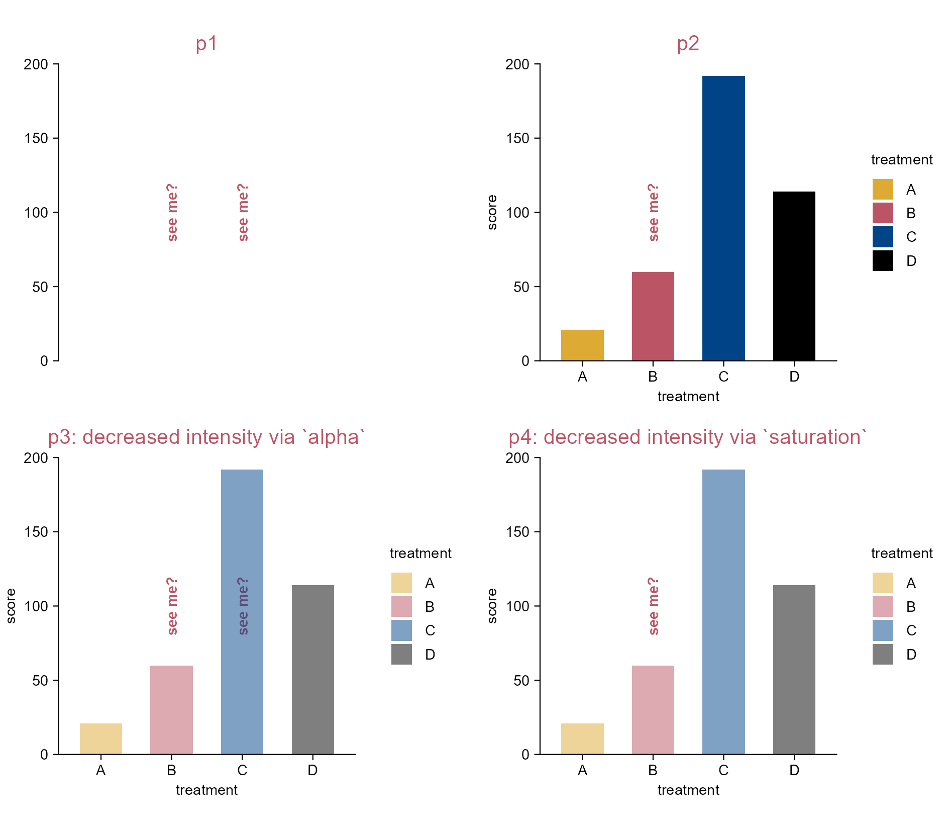
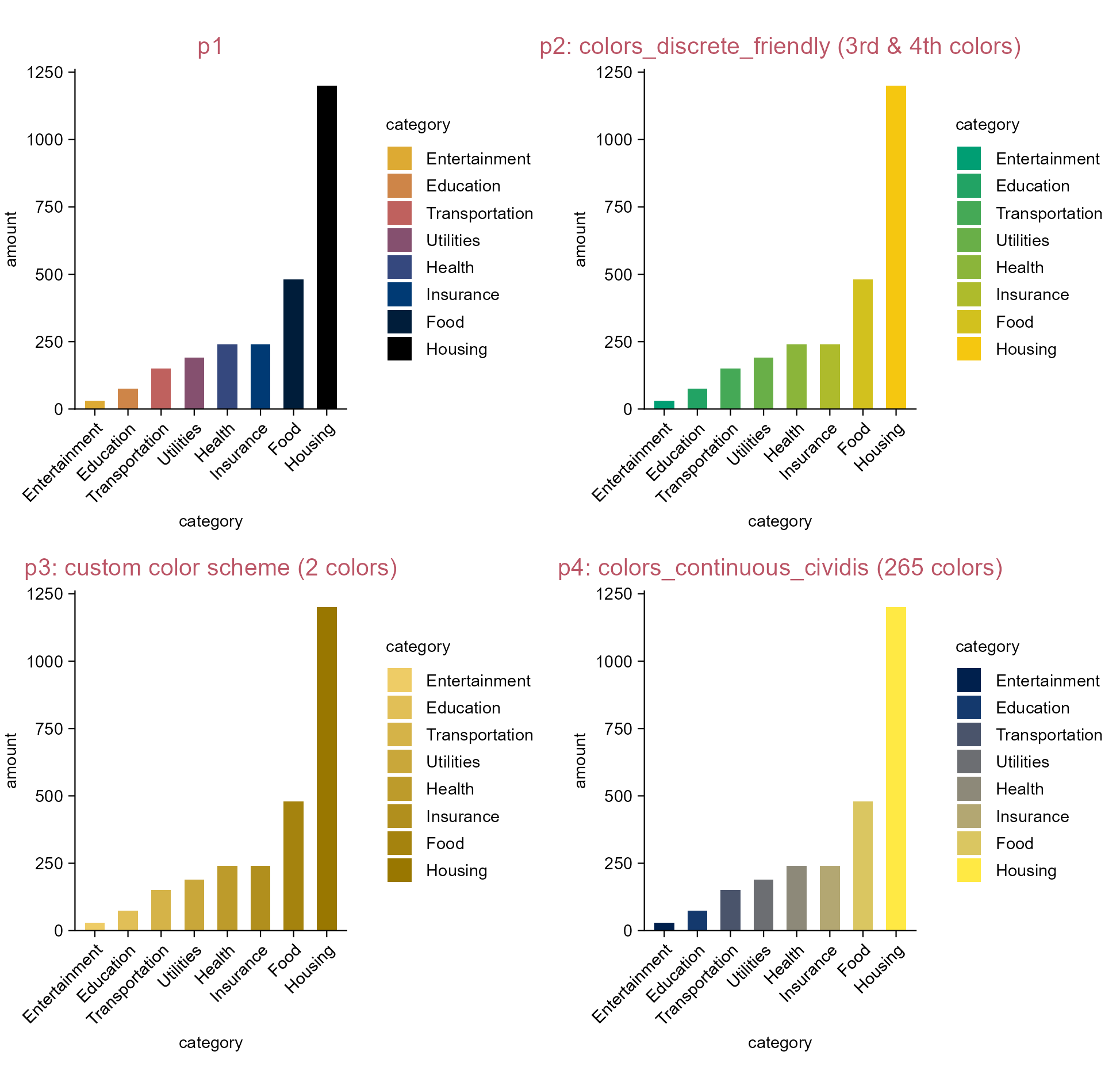
3.22 Change color scheme (e.g. bar plot)
library(tidyplots)# View top 10 rows of the columns usedspendings |> dplyr::select(category, amount) |> dplyr::slice_head(n =10)
Tidyplots comes with a number of default color schemes.
A color scheme (default or custom) might contain limited number of colors (e.g. p3), tidyplots will automatically fill up the gaps between colors to deliver exactly the number that is required for the plot.
Similarly, when a color scheme contains more colors than needed (e.g. p4), tidyplots will select the required number of colors by attempting to evenly sample from the supplied color vector.
Change the color scheme.
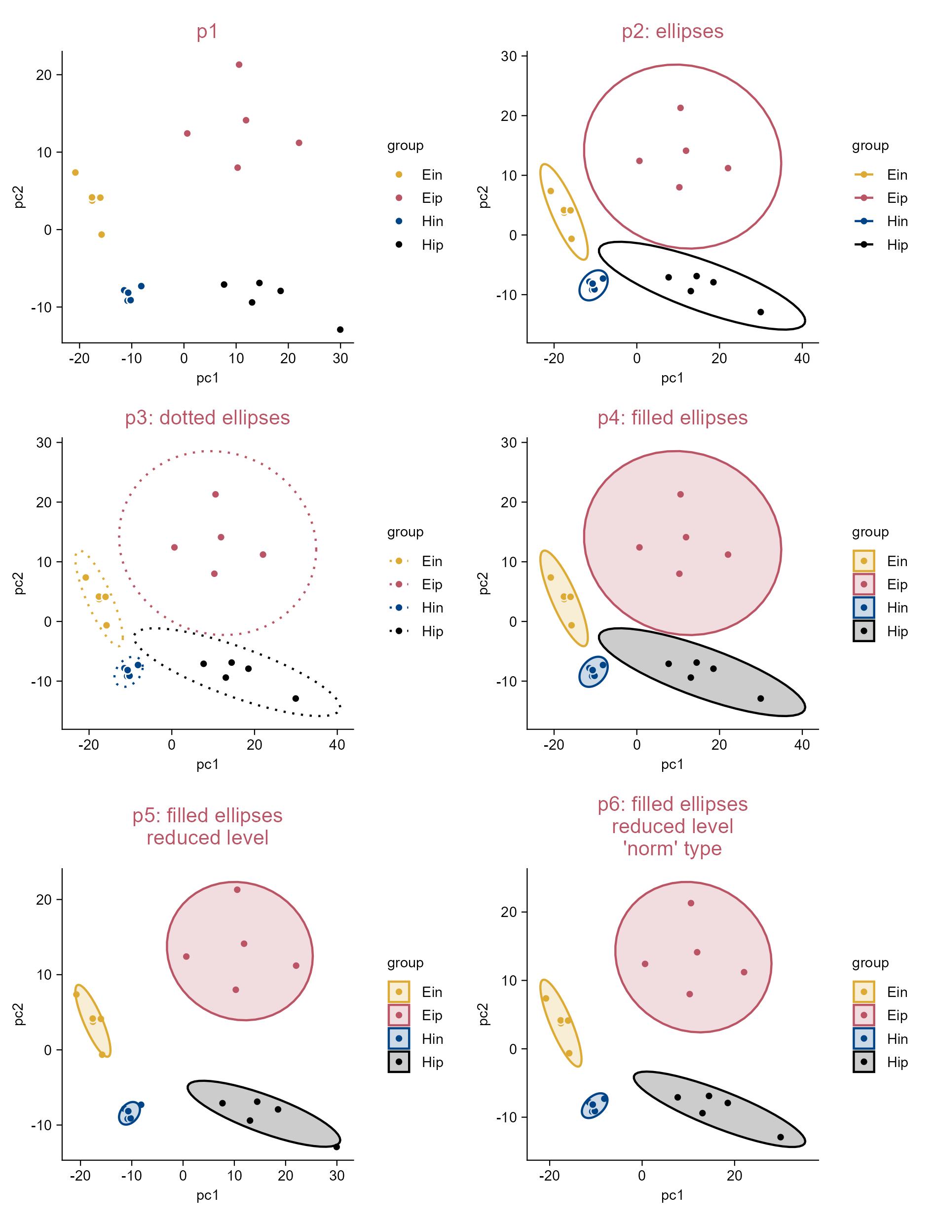
3.23 Add data ellipses (e.g. dot plot)
library(tidyplots)# View top 10 rows of the columns usedpca |> dplyr::select(pc1, pc2, group) |> dplyr::slice_head(n =10)
# A tibble: 10 × 3
pc1 pc2 group
<dbl> <dbl> <chr>
1 -10.8 -9.17 Hin
2 -11.5 -7.84 Hin
3 -10.2 -9.11 Hin
4 -8.18 -7.30 Hin
5 -10.7 -8.15 Hin
6 -17.6 3.75 Ein
7 -20.8 7.37 Ein
8 -15.8 -0.644 Ein
9 -17.6 4.16 Ein
10 -16.0 4.13 Ein
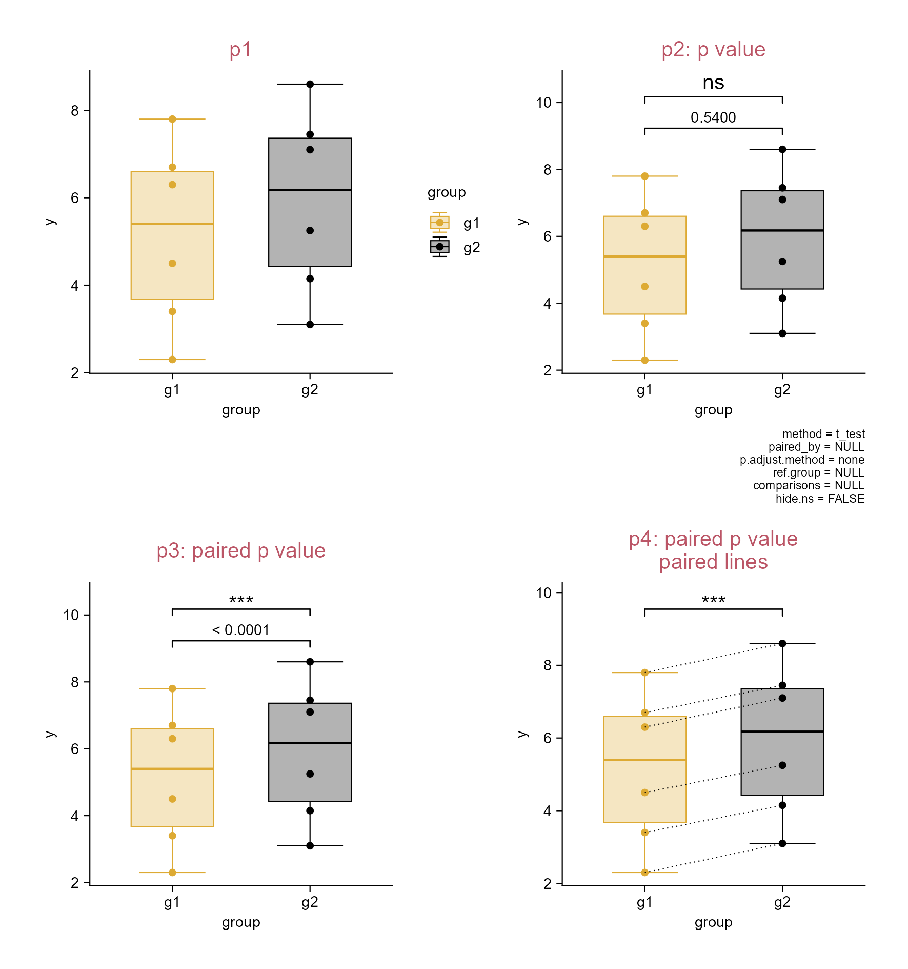
library(tidyplots)# View top 10 rows of the columns usedstudy |> dplyr::select(group, score, dose, treatment) |> dplyr::slice_head(n =10)
# A tibble: 10 × 4
group score dose treatment
<chr> <dbl> <chr> <chr>
1 placebo 2 high A
2 placebo 4 high A
3 placebo 5 high A
4 placebo 4 high A
5 placebo 6 high A
6 placebo 9 low B
7 placebo 8 low B
8 placebo 12 low B
9 placebo 15 low B
10 placebo 16 low B
p1 <- study |>tidyplot(x = group, y = score, color = dose) |>add_boxplot() |>add_data_points() |>add_title(title ="p1")p2 <- p1 |>adjust_title(title ="p2: test asterisks") |>add_test_asterisks()p3 <- p1 |>adjust_title(title ="p3: test p value") |>add_test_pvalue(hide_info =TRUE)p4 <- study |>tidyplot(x = treatment, y = score, color = treatment) |>add_boxplot() |>add_data_points() |>add_test_asterisks(hide_info =TRUE) |>add_title(title ="p4: test asterisks")
Because tidyplots is based on ggplot2 … thereby, tidyplots provides access to a wide range of features that are implemented within ggplot2 or ggplot2 extension packages … add() helper function.
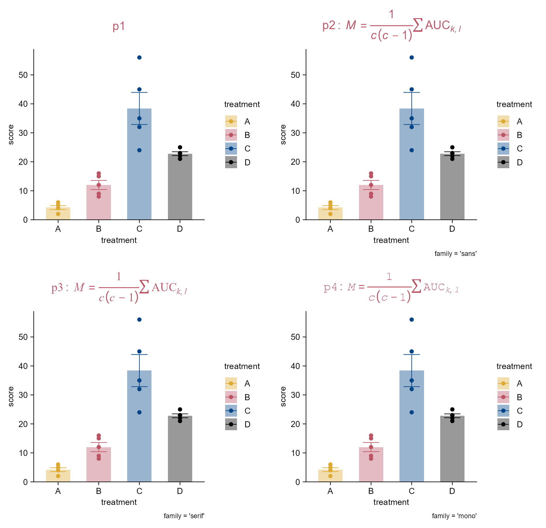
library(tidyplots)# View top 10 rows of the columns usedstudy |> dplyr::select(treatment, score) |> dplyr::slice_head(n =10)
# A tibble: 10 × 2
   treatment score
   <chr>     <dbl>
 1 A             2
 2 A             4
 3 A             5
 4 A             4
 5 A             6
 6 B             9
 7 B             8
 8 B            12
 9 B            15
10 B            16
For the title of p4: “p4: M. tuberculosis” is followed by clicking Space bar twice and Enter button once, then followed with “via ggtext::element-markdown()”.
Add ggplot2 (extensions) code.
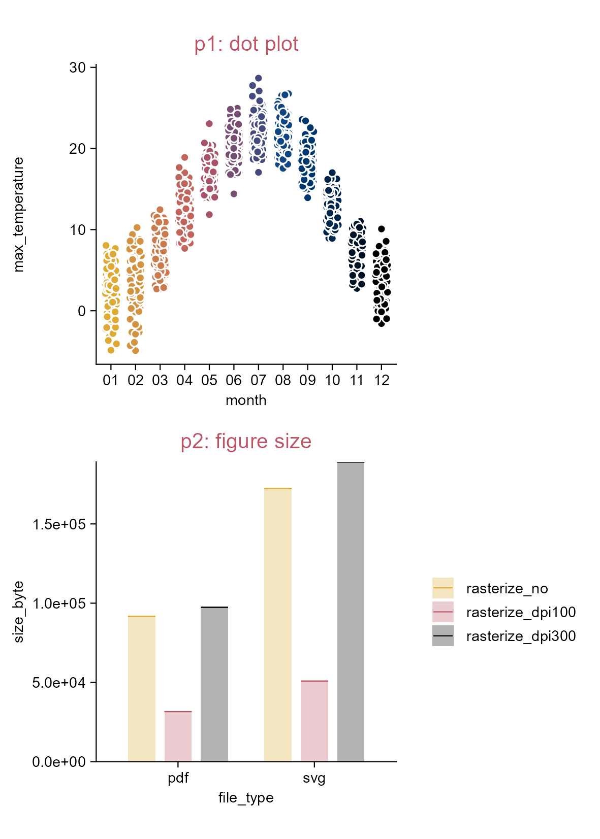
3.34 Add ggplot2 (extention) code (three more plots)
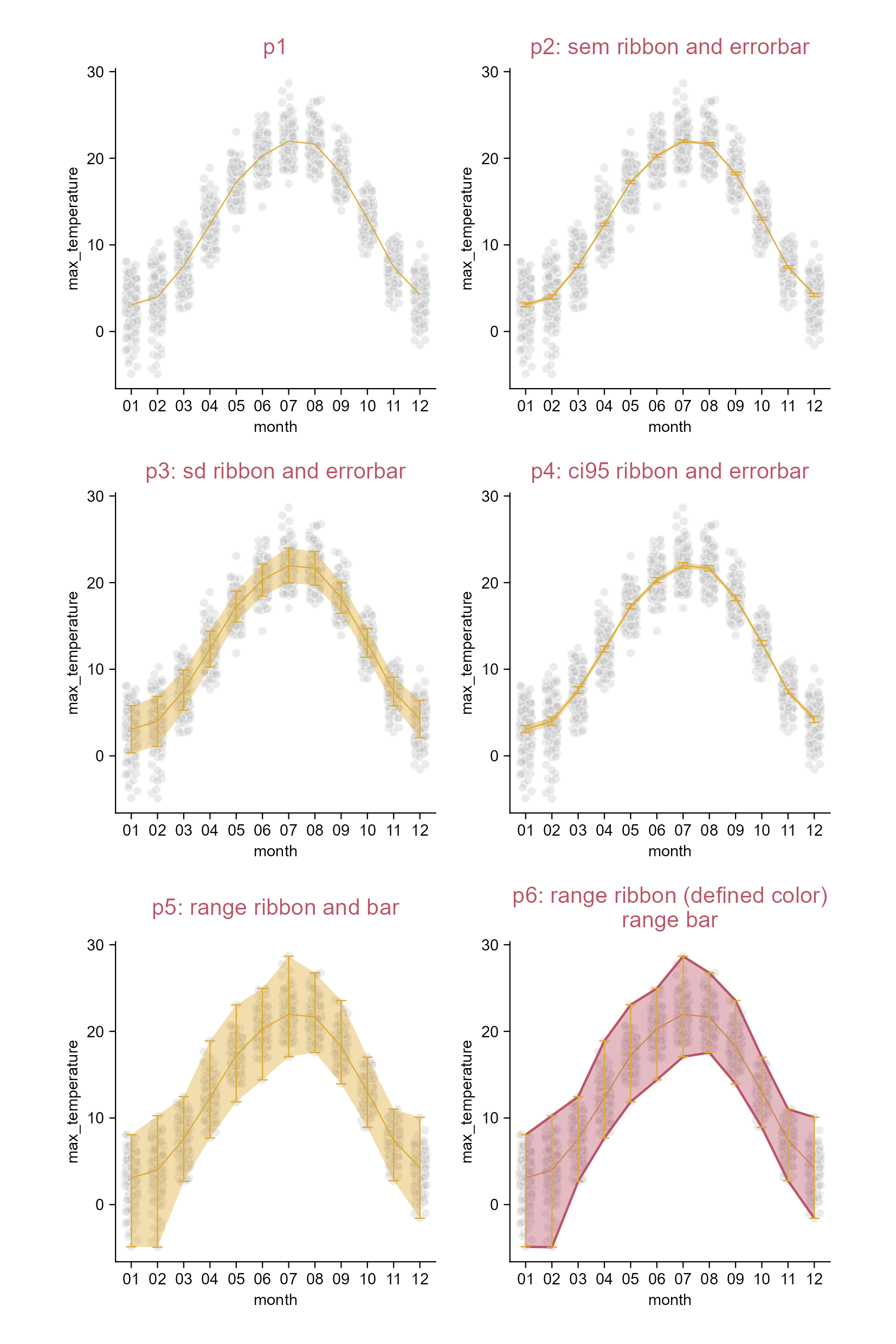
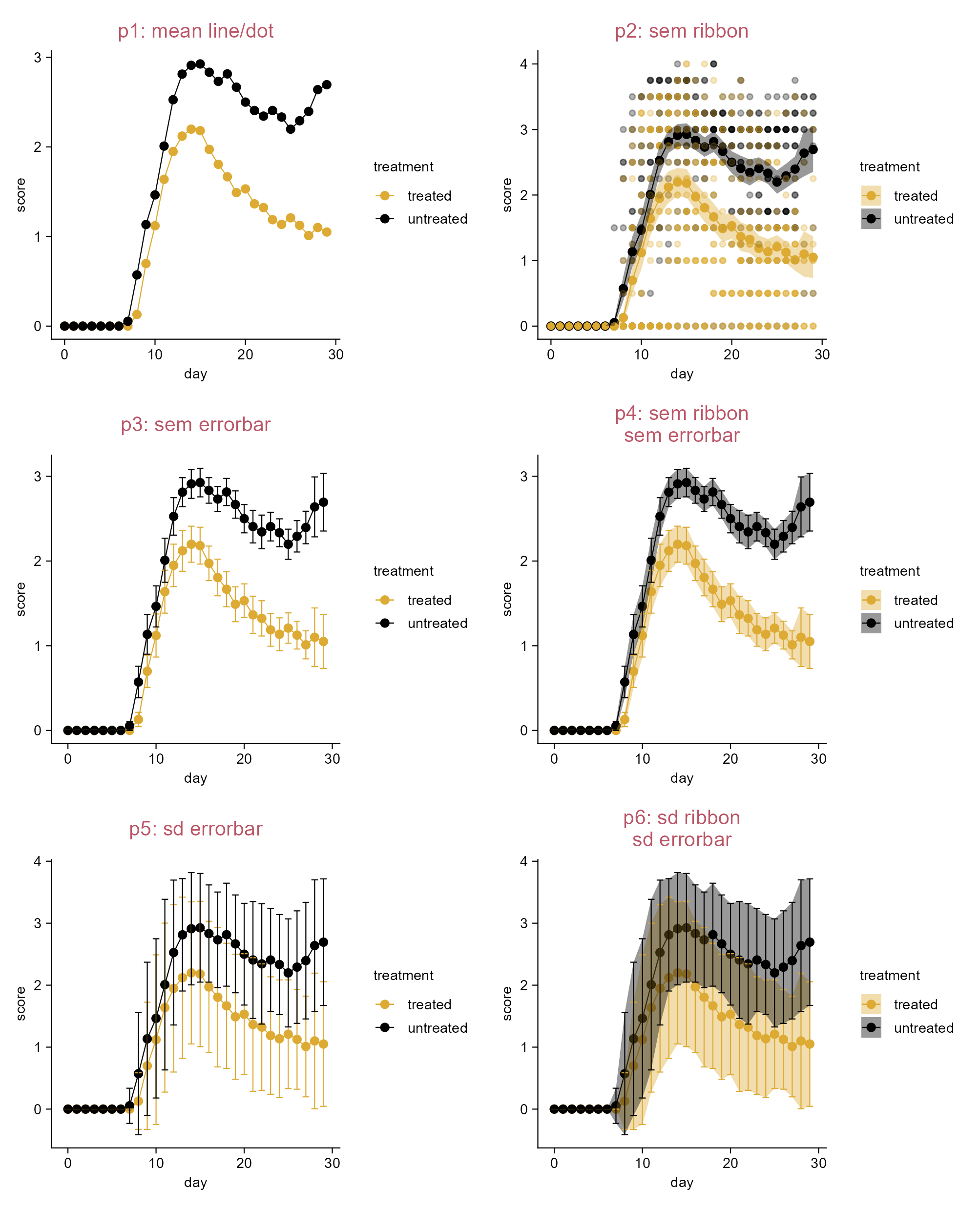
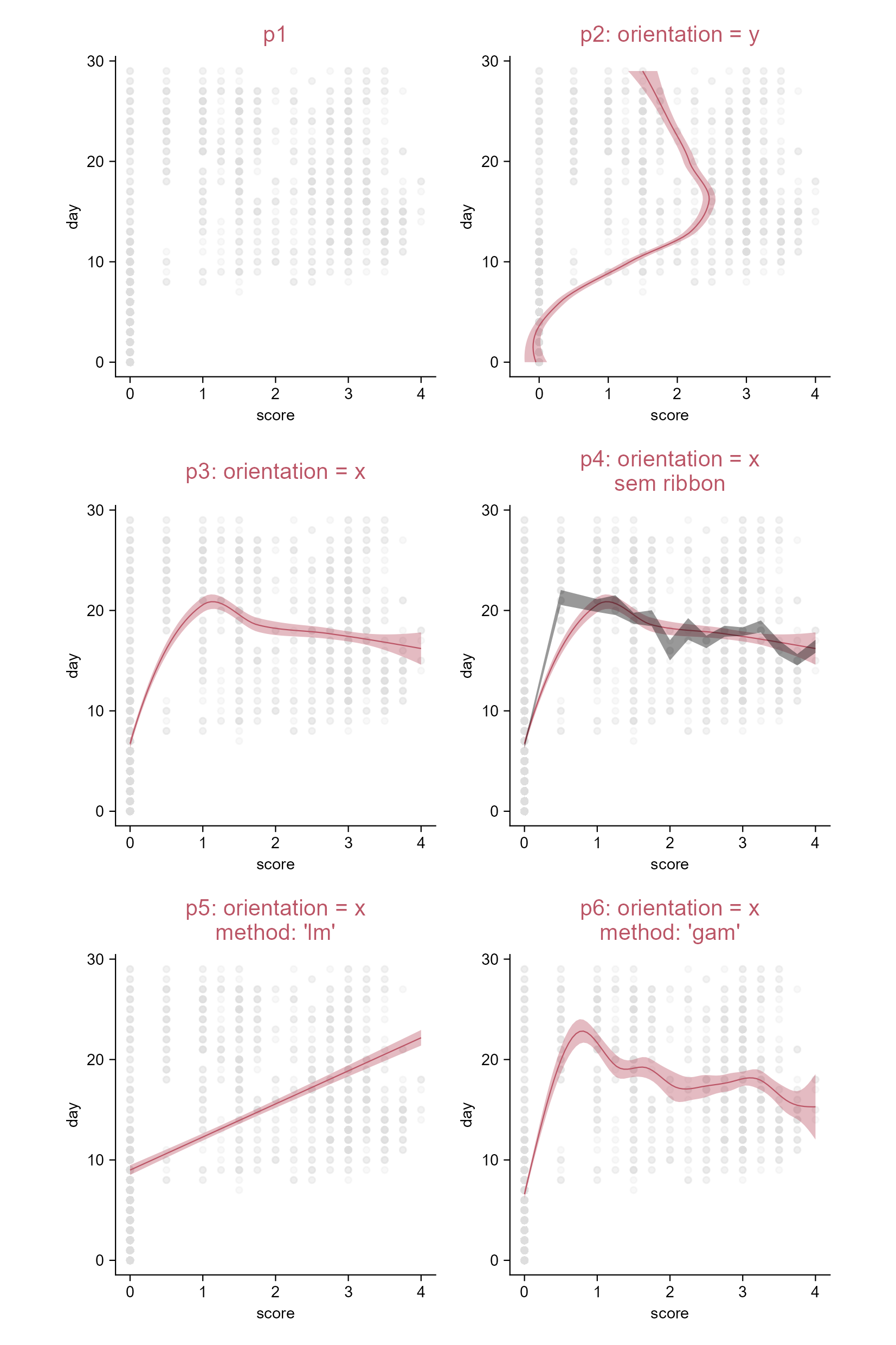
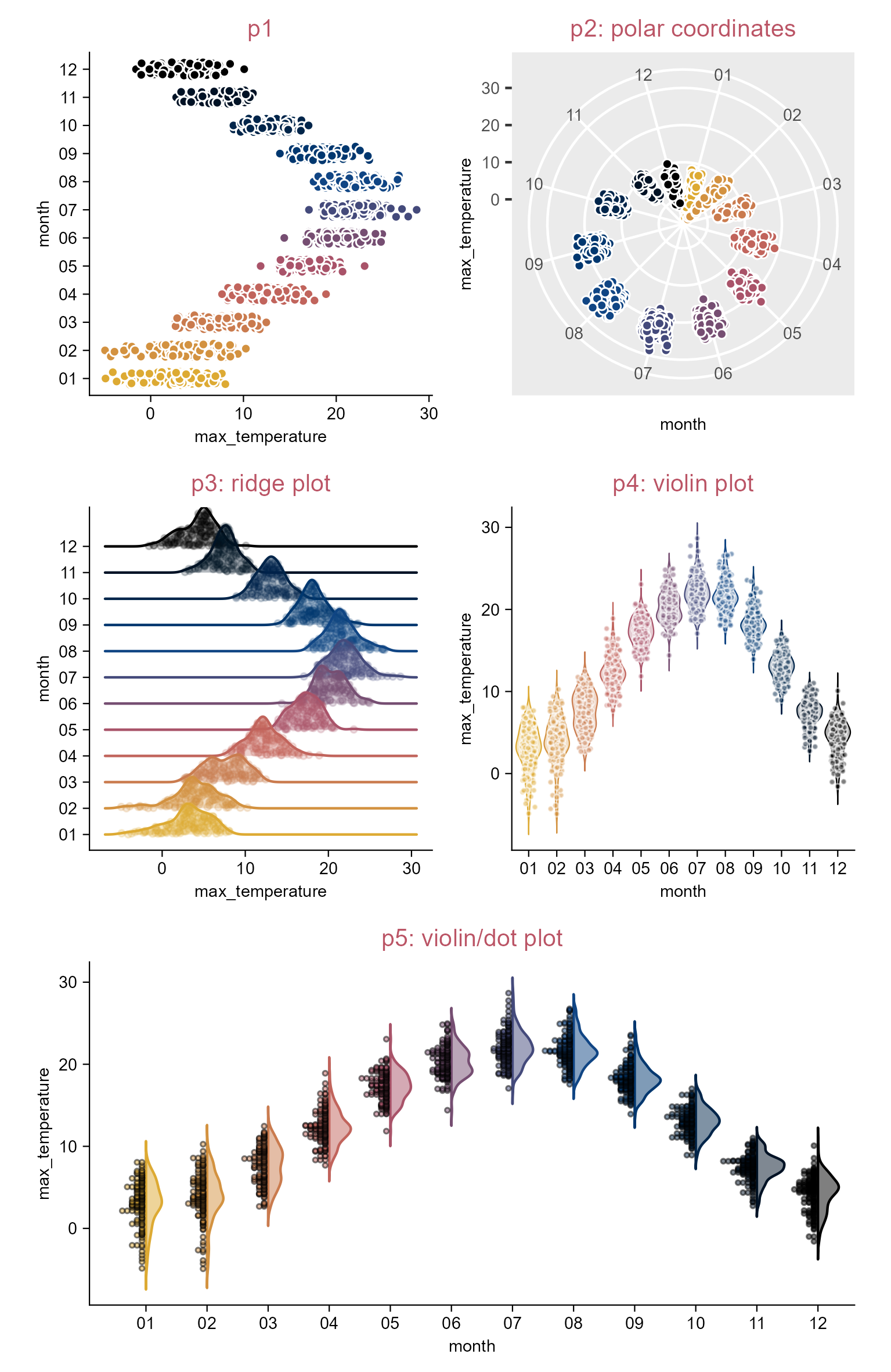
library(tidyplots)# View top 10 rows of the columns usedclimate |> dplyr::select(max_temperature, month) |> dplyr::slice_head(n =10)
Tidyplots is easier for many common plotting tasks.
For more complex plots, you can either augment tidyplots with custom ggplot2 code using the add() function or switch to ggplot2 for full flexibility.
Add ggplot2 (extensions) code.
3.35 Save multiple formats by piping through (e.g. dot plot)
library(tidyplots)# Viewstudy
# A tibble: 20 × 7
treatment group dose participant age sex score
<chr> <chr> <chr> <chr> <dbl> <chr> <dbl>
1 A placebo high p01 23 female 2
2 A placebo high p02 45 male 4
3 A placebo high p03 32 female 5
4 A placebo high p04 37 male 4
5 A placebo high p05 24 female 6
6 B placebo low p06 23 female 9
7 B placebo low p07 45 male 8
8 B placebo low p08 32 female 12
9 B placebo low p09 37 male 15
10 B placebo low p10 24 female 16
11 C treatment high p01 23 female 32
12 C treatment high p02 45 male 35
13 C treatment high p03 32 female 24
14 C treatment high p04 37 male 45
15 C treatment high p05 24 female 56
16 D treatment low p06 23 female 23
17 D treatment low p07 45 male 25
18 D treatment low p08 32 female 21
19 D treatment low p09 37 male 22
20 D treatment low p10 24 female 23
# Plot and savestudy |>tidyplot(x = group, y = score, color = dose) |>add_data_points_beeswarm() |>add_sem_errorbar() |>save_plot("images/multiple-formats-via-pipe.pdf", view_plot =FALSE) |>save_plot("images/multiple-formats-via-pipe.png", view_plot =FALSE) |>save_plot("images/multiple-formats-via-pipe.svg", view_plot =FALSE)
Save a plot in multiple formats by piping through.
3.36 Save multiple PDFs by piping through (e.g. violin plot)
library(tidyplots)# View top 10 rows of the columns usedgene_expression |> dplyr::select( group, expression, condition, sample_type, is_immune_gene) |> dplyr::slice_head(n =10)
# A tibble: 10 × 5
group expression condition sample_type is_immune_gene
<chr> <dbl> <chr> <chr> <chr>
1 Hin 2.20 healthy input no
2 Hin 2.20 healthy input no
3 Hin 2.66 healthy input no
4 Hin 2.65 healthy input no
5 Hin 3.44 healthy input no
6 Ein 5.03 disease input no
7 Ein 5.31 disease input no
8 Ein 5.37 disease input no
9 Ein 5.54 disease input no
10 Ein 5.65 disease input no
3.37 Save multiple PDFs at once (e.g. violin plot)
library(tidyplots)# View 10 rows of the columns usedgene_expression |> dplyr::select( group, expression, external_gene_name) |> dplyr::slice(c(1:2, 101:102, 201:202, 301:302, 401:402))
# A tibble: 10 × 3
group expression external_gene_name
<chr> <dbl> <chr>
1 Hin 2.20 Apol6
2 Hin 2.20 Apol6
3 Hin 7.39 Vgf
4 Hin 6.86 Vgf
5 Hin 8.21 Dpf2
6 Hin 8.29 Dpf2
7 Hin 5.87 Ankrd54
8 Hin 5.62 Ankrd54
9 Hin 7.84 Fam96b
10 Hin 7.52 Fam96b
# Plot and savegene_expression |>tidyplot(x = group, y = expression, color = group) |>add_violin(trim =FALSE) |>add_data_points_beeswarm(white_border =TRUE) |>adjust_size(overall_width =100) |># see the note of next pageadjust_theme_details(strip.text.x.top = ggplot2::element_text(face ="italic")) |># gene names in italicsplit_plot(by = external_gene_name, ncol =2, nrow =2) |>save_plot("images/multiple-pdf-at-once.pdf", multiple_files =TRUE, view_plot =FALSE)
The overall_width and overall_height parameters of the adjust_size() function control the overall dimensions of a multiplot layout generated with split_plot().
The function adjust_theme_details() is a wrapper around ggplot2::theme().
3.38 Save intermediate stages (e.g. bar plot)
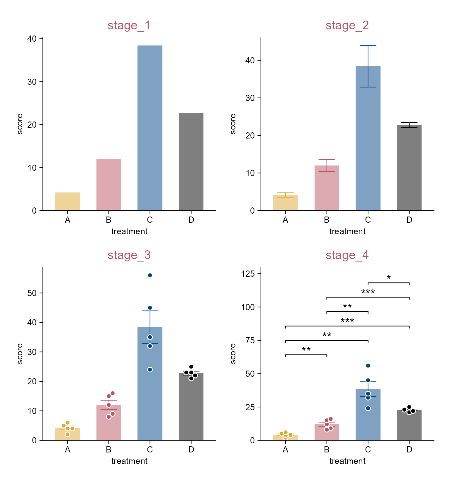
library(tidyplots)# View top 10 rows of the columns usedstudy |> dplyr::select(treatment, score) |> dplyr::slice_head(n =10)
# A tibble: 10 × 2
   treatment score
   <chr>     <dbl>
 1 A             2
 2 A             4
 3 A             5
 4 A             4
 5 A             6
 6 B             9
 7 B             8
 8 B            12
 9 B            15
10 B            16
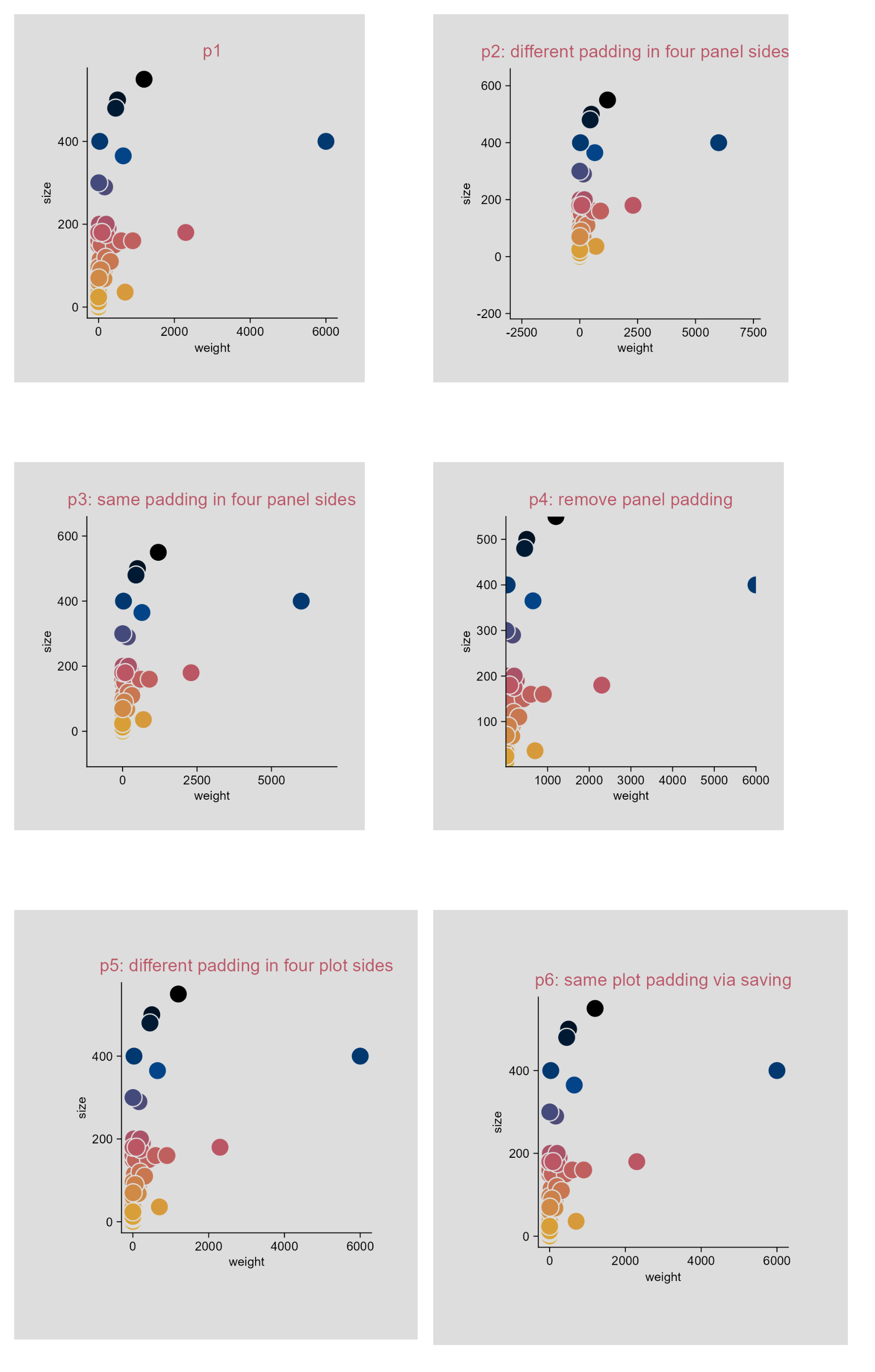
# Plotp1 <- animals |>tidyplot(x = weight, y = size, color = size, paper ="#dddddd") |>add_data_points(white_border =TRUE, size =3) |>add_title(title ="p1") |>remove_legend()p2 <- p1 |>adjust_title(title ="p2: different padding in four panel sides") |>adjust_padding(top =0.2, right =0.3, bottom =0.4, left =0.5)p3 <- p1 |>adjust_title(title ="p3: same padding in four panel sides") |>adjust_padding(all =0.2)p4 <- p1 |>adjust_title(title ="p4: remove panel padding") |>remove_padding()p5 <- p1 |>adjust_title(title ="p5: different padding in four plot sides") |>adjust_theme_details(plot.margin = ggplot2::margin(t =0.5, r =0.5, b =1, l =1, unit ="cm"))p6 <- p1 |>adjust_title(title ="p6: same plot padding via saving") |>save_plot("images/plot_panel_padding_p6.png", padding =0.3) # defaults to 0.1 meaning 10%
Panel and plot padding.
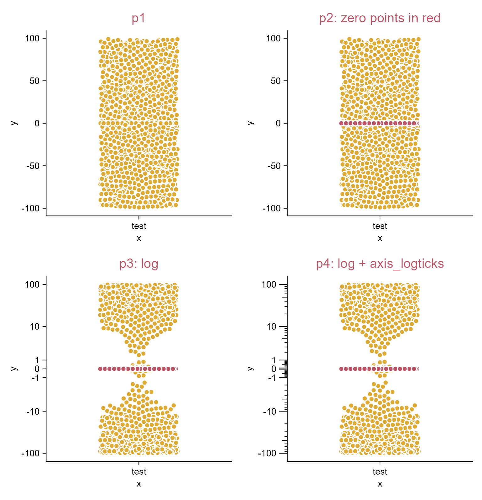
3.40 Use a log10 axis for data containing zero and negative values (e.g. dot plot)
library(tidyplots)set.seed(42)y <-runif(n =500, min =0, max =100)# change 30 values to zeroy[sample(NROW(y), size =30)] <-0df <- tibble::tibble(x ="test", y =c(y, y *-1))# View rows 496 - 505df |> dplyr::slice(496:505)
# A tibble: 10 × 2
   x          y
   <chr>  <dbl>
 1 test   18.3
 2 test    0
 3 test   30.5
 4 test   16.6
 5 test    3.28
 6 test  -91.5
 7 test  -93.7
 8 test  -28.6
 9 test  -83.0
10 test  -64.2